In this post, I'm going to talk about how I calibrated the accelerometer in my bot. The calibration finds the relationship between measured acceleration and robot speed.
Some definitions
Measured acceleration comes into the processor in units of "LSB", or least significant bits. It's a jargon-y term that basically means raw data. We can convert LSB to g's by finding how many LSB are in the full-scale range of the accelerometer, then dividing by the full scale. But it's an unnecessary step since in the end we don't care about g's. We're going to directly relate LSB to robot speed.
As discussed in the previous post, we are expressing speed in terms of microseconds per degree to allow for more integer math. Here is what our angle calculation looks like:

Where robotPeriod is our measurement, in microseconds per degree. The purpose of this calibration is to find the relationship between accelerometer LSBs and microseconds per degree.
The calibration method
We will define the relationship between accelerometer data and microseconds per degree by taking twin measurements from a real-world test. I use the test stand from part 6 to hold the bot, and then I slowly spin up and down the bot.
Meanwhile, the bot is measuring accelerometer data and beacon edge times. Beacon edge times tell us pretty directly our microseconds/degree, since they are measured in microseconds and we know our edges are 360 degrees apart. If you don't have a beacon on your bot, you can substitute with an optical tachometer.
Our bot decomposes the data and sends it to the controller (this is why we used XBee's as our radios).
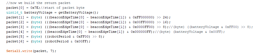
robotPeriod in this case represents our raw accelerometer measurement
On the controller side, we recompose the data, and send it to my computer over the usb cable.
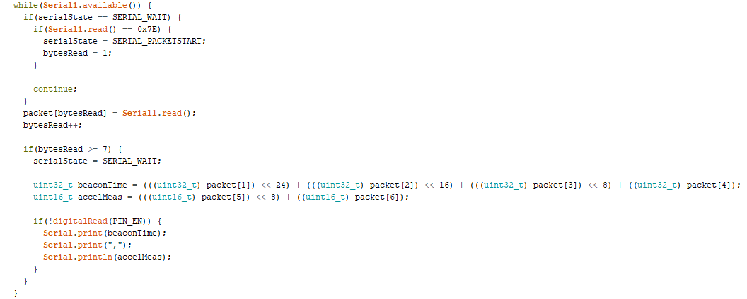
You can also do this by having a third XBee plugged into your computer via an XBee explorer, I just didn't happen to have one lying around.
On the host computer, I have a python script running that pulls in the data. It doesn't do much but put it into a file for later.

I spun the bot up and down a couple times, and then shut down the test. Next, I wrote another python script to parse the data. Here are the points I gathered:

As you can see, there are some good curves, but lots of artifacts! We will filter those artifacts out here. In the final code, the accelerometer and the beacon will work together to filter those out in real time.
Some easy artifacts to filter out include the ones at y=0 (when the accelerometer is reporting data but the beacon isn’t) and the ones at y= very large (which happens when the beacon misses several rotations. We add a simple high and low cutoff to filter those.

Now we see the relationship we are looking for much more clearly. But, it’s in triplicate here. Every duplicate is due to the beacon missing N rotations. If the beacon missed every other edge, the us/deg would be double. If it missed twice in a row, triple, and so on.
We need to remove the duplicate curves, as they aren’t useful to us. To do this, we will use a piecewise linear cutoff.

The last artifact is the little “wing” at y=400. This one actually stumps me, I don’t know where it’s from. We’ll add an extra filter and move on…

That looks much better. We need to use curve fitting to find the closest equation to represent this curve. Luckily, python can do that too!
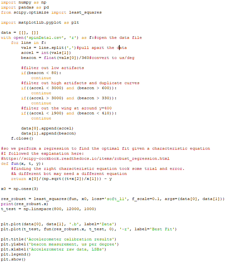

That looks pretty good! Lets take a look at the coefficients it gave us:

This makes our equation:

Ouch, that is pretty ugly. Luckily it only needs to run every time we get a new accelerometer measurement. And if it ends up being too slow in the future, we can use a lookup table instead.
Here is how the bot performs with the above equation and the improved accelerometer algorithm: