Magnetometers: Software Implementation

I’m using this post as a way to write down all of the ideas of how to implement our accelerometer informed adaptive sample rate magnetometer with Goertzel’s analysis. Or, how about we call it Meltycompass.

This post was published early in service of a review. While the majority of it is solid, there is still an unidentified flaw preventing correct operation. You’ve been warned.

You can find the source code associated with this post here.

We’re going to do everything in our power to reduce our computational load, but we’re still running on an RP2040. With a relatively low clock rate and no hardware floating point, we can easily max it out.

But the RP2040 does have the benefit of a second core, which until now has been completely unused. We will dedicate this second core to running our heading sensor.

Our overall plan of attack is pictured below.

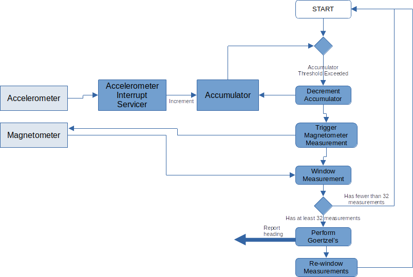
Planned software block diagram

Accelerometer Handling

The H3LIS331DL can be configured to self-trigger at 1000Hz and toggle a pin every time a new measurement is ready. So we will use a GPIO interrupt to read our data.

void accelInterrupt(uint gpio, uint32_t events) {
    headingSensor.serviceAccelInterrupt();
    gpio_acknowledge_irq(gpio, events);
}

void core1_main() {
    gpio_init(GPIO_ACCEL_INT);
    gpio_set_dir(GPIO_ACCEL_INT, false);

    gpio_set_irq_enabled_with_callback(GPIO_ACCEL_INT, GPIO_IRQ_EDGE_RISE, true, accelInterrupt);

The SPI protocol is handled by the PIO rather than the hard SPI peripheral. After attempting use, I realized the RP2040’s hard SPI peripheral isn’t that great. The interrupt support is poor, and it can’t hold CSn low across words. I started with the example SPI PIO program, and modified the CSn timings slightly.

.program spi_cpha0_cs
.side_set 2

.wrap_target
bitloop:
    out pins, 1        side 0x0 [1]
    in pins, 1         side 0x1
    jmp x-- bitloop    side 0x1

    out pins, 1        side 0x0
    mov x, y           side 0x0     ; Reload bit counter from Y
    in pins, 1         side 0x1
    jmp !osre bitloop  side 0x1     ; Fall-through if TXF empties

    nop                side 0x1 [1] ; CSn back porch
public entry_point:                 ; Must set X,Y to n-2 before starting!
    pull ifempty       side 0x3 [1] ; Block with CSn high (minimum 2 cycles)
                                    ; Note ifempty to avoid time-of-check race
    nop                side 0x1 [1] ; Drop CSn before SCK
.wrap

Accumulator: Timing Our Magnetometer Measurements

The maximum sample rate of our magnetometer is 300Hz. We can always sample slower, but not faster, so this max speed must occur at the top of our signal frequency range. Signal frequency is the same as our rotation speed, so basically we need to pick a top speed. At that top speed, we sample the magnetometer at maximum.

For our robots, we are generally around 1300RPM. So lets pick 1500RPM as our max. That corresponds to 25Hz. So when we are spinning at 25Hz, we need to sample at 300Hz.

The way to handle this with the least overhead is a simple accumulator. When we get an accelerometer measurement, add it to a variable (the accumulator). When the accumulator reaches a threshold, subtract the threshold from it and trigger a measurement. Set up this way, if we spin half as fast, the accumulator gains value half as fast. So our magnetometer will trigger half as fast. Exactly the behavior we want.

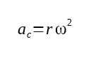
Now, this assumes that the response from the accelerometer is linear. But that isn’t true by default, because centripetal acceleration has a square relationship with rotation speed.

$$ a_c = r\omega^2 $$

So to correct this, we will need to use the square root of our measurement.

$$\omega = \sqrt{\frac{a_\textrm{meas}}{r}}$$

Additionally, we will need to convert from raw accelerometer LSBs to acceleration.

$$a(x)=\frac{\textrm{Sample}(x)\times9.8G_\textrm{max}}{2^{\textrm{bits}-1}}$$

Putting this all together:

$$\omega(x) = \sqrt{\frac{9.8G_\textrm{max}}{r2^{\textrm{bits}-1}}} \sqrt{\textrm{Sample(x)}}$$

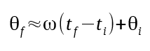
Another way to look at this is we use the accelerometer to ensure that exactly the same rotational distance is covered between every magnetometer sample. We can calculate what that distance is using known constants.

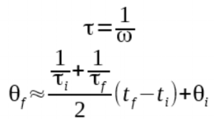
$$\theta = \frac{\omega_{\textrm{max}}}{f_\textrm{mag max}}$$

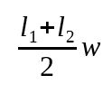
Bringing back math from previous blog posts, we can also calculate how far we’ve traveled by integrating our speed as measured by the accelerometer.

$$\theta = \int_0^{T_\textrm{mag}}\omega(t)dt$$

Since we have rotational speed in the form of discrete measurements, we must replace our continuous integral with an approximation. We will use triangular approximation.

$$\theta = \int_{0}^{T_\textrm{mag}}\omega(t)dt \approx \sum_{i=1}^{n}\frac{\omega(i)+\omega(i-1)}{2}T_\textrm{accel}$$

This approximation will of course introduce error. But unlike accelerometer-only algorithms, the error is only relevant to a single magnetometer measurement and “resets” afterwards. So it has much less time to build up. Lets bring our equations together.

$$\frac{\omega_{\textrm{max}}}{f_\textrm{mag max}} \approx \sum_{i=1}^{n}\frac{\omega(i)+\omega(i-1)}{2}T_\textrm{accel}$$

The left side of that equation is precomputed, and the contents of the sum must be calculated for every accelerometer sample. So any math that can be moved to the left side makes our code faster.

$$\frac{2f_\textrm{accel}\omega_{\textrm{max}}}{f_\textrm{mag max}} \approx \sum_{i=1}^{n}\omega(i)+\omega(i-1)$$

Now we pull in our conversion from LSBs to $\omega$.

$$\frac{2f_\textrm{accel}\omega_{\textrm{max}}}{f_\textrm{mag max}} \approx \sqrt{\frac{9.8G_{max}}{2^{\textrm{bits}-1}r}} \sum_{i=1}^{n} \sqrt{\textrm{Sample}(i)}+\sqrt{\textrm{Sample}(i-1)}$$

And finally:

$$\frac{4\pi f_\textrm{accel}f_{\textrm{bot max}}}{f_\textrm{mag max}} \sqrt{\frac{2^{\textrm{bits}-1}r}{9.8G_{max}}} \approx \sum_{i=1}^{n} \sqrt{\textrm{Sample}(i)}+\sqrt{\textrm{Sample}(i-1)}$$

The final equation compares a sum of accelerometer measurements to a fixed threshold. When the sum and threshold match, it is time to take a magnetometer measurement.

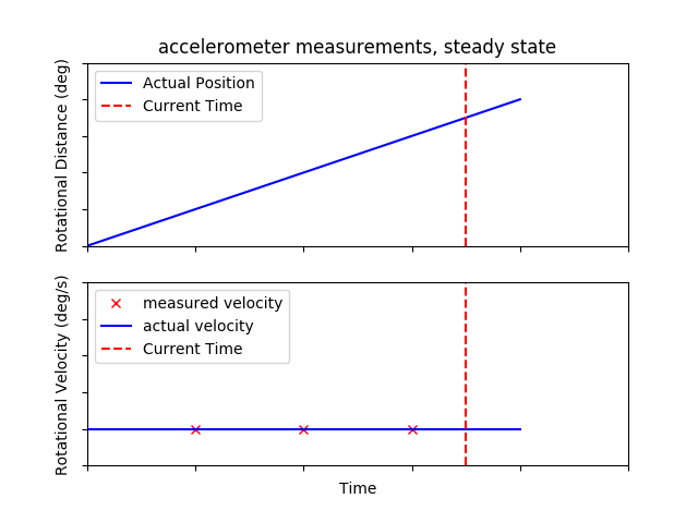
Timing between accelerometer samples

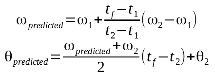
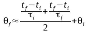
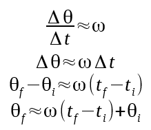
If we rely only on accelerometer measurements, at best we could trigger our magnetometer measurements with a precision of 1ms. To do better, we will perform a linear extrapolation from the previous two samples.

We will accept some error for a simplification, and assume that the average acceleration between the previous two points is constant.

Starting from an earlier equation, we add an extra term to make the equality exact.

$$\frac{\omega_{\textrm{max}}}{f_\textrm{mag max}} = \sum_{i=1}^{n}\frac{\omega(i)+\omega(i-1)}{2}T_\textrm{accel} + \frac{\omega_\textrm{Predicted}+\omega(i)}{2}t$$

Where “t” is the duration of our extra partial period. Simplify down a bit:

$$\frac{ 2 f_\textrm{accel} \omega_\textrm{max} } {f_\textrm{mag max}} = \sum_{i=1}^{n}(\omega(i)+\omega(i-1)) + (\omega_\textrm{Predicted} + \omega(i)) \frac{t}{ T_\textrm{accel} }$$

We convert from $\omega$ to samples:

$$\frac{4\pi f_\textrm{accel}f_{\textrm{bot max}}}{f_\textrm{mag max}}\sqrt{\frac{2^{\textrm{bits}-1}r}{9.8G_{max}}} = \sum_{i=1}^{n}( \sqrt{\textrm{Sample}(i)}+\sqrt{\textrm{Sample}(i-1)})$$ $$ + (\sqrt{\textrm{Sample}(\textrm{predicted})} + \sqrt{\textrm{Sample}(i)})\frac{t}{T_\textrm{accel}}$$

The equation is starting to get out of hand, so lets redefine it in this form:

$$\textrm{Threshold} = \textrm{Accumulation} + \textrm{Prediction}$$ $$\textrm{Threshold} = \frac{4\pi f_\textrm{accel}f_{\textrm{bot max}}}{f_\textrm{mag max}}\sqrt{\frac{2^{\textrm{bits}-1}r}{9.8G_{max}}}$$ $$\textrm{Accumulation} = \sum_{i=1}^{n}( \sqrt{\textrm{Sample}(i)}+\sqrt{\textrm{Sample}(i-1)})$$

"Threshold" is composed of known constants only, so it can and should be precomputed. "Accumulation" is composed entirely of real accelerometer data. It should be incremented by the accelerometer interrupt, and be zeroed (actually, "Threshold" should be subtracted from it) after a magnetometer sample is taken. Now we have to finish deriving our "Prediction" term.

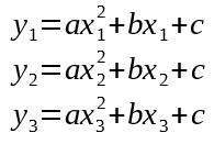
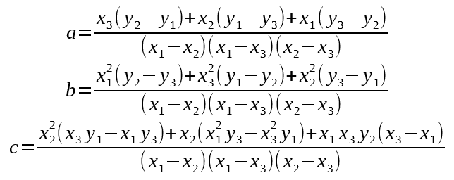
We assume a fixed slope for $\sqrt{\textrm{Sample}(x)}$, which we can find by:

$$m = \frac{\sqrt{\textrm{Sample}(i)} - \sqrt{\textrm{Sample}(i-1)}}{T_\textrm{accel}}$$

Given a fixed slope, our predicted sample takes the form of $y=mx+b$.

$$\textrm{Predicted Val} = \frac{\sqrt{\textrm{Sample}(i)} - \sqrt{\textrm{Sample}(i-1)}}{T_\textrm{accel}} t + \sqrt{\textrm{Sample}(i)}$$

Lets put this all together.

$$\textrm{Prediction} = \frac{ \frac{\sqrt{\textrm{Sample}(i)} - \sqrt{\textrm{Sample}(i-1)}}{T_\textrm{accel}} t + 2\sqrt{\textrm{Sample}(i)} }{T_\textrm{accel}} t$$

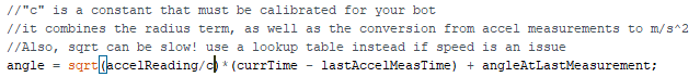
We pre-calculate most of the values we need in the accelerometer interrupt.

void MeltyCompass::serviceAccelInterrupt() {
    //Spin mode: update the accumulator and extrapolation values
    if(mEnable) {
        mLastAccelSampleTime = time_us_32();
        uint32_t accelSample = (uint32_t) (mAccel->getSample());
        accelSample = squareRootRounded(accelSample);
        mAccelAccumulator += accelSample + mLastAccelSample;
        mAccumulatorRise = accelSample - mLastAccelSample;
        mLastAccelSample = accelSample;

    //Non-spin mode: get the current orientation
    } else {
        int16_t accelSample = mAccel->getSample() + 11;
        mOrientation = accelSample > 0;
    }
}

And here is the loop where we wait to trigger our magnetometer measurement.

while(mEnable) {
    uint32_t extraTime = time_us_32()-mLastAccelSampleTime;
    uint32_t predictedAccumulation = 
        (2*mLastAccelSample + (mAccumulatorRise*extraTime)/ACCEL_SAMPLE_PERIOD)
        * extraTime / ACCEL_SAMPLE_PERIOD;

    if(mAccelAccumulator + predictedAccumulation >= ACCUMULATION_THRESH) {
        //We subtract the threshold from the accumulator later
        //while we update with the new heading value
        break;
    }
}

Goertzel Coefficients

Normally when using Goertzel’s, you will calculate Goertzel coefficients to match your sampled data. For our use, that is flipped. We will be warping our data to match pre-chosen Goertzel coefficients. So our coefficients are based off of the setpoint of our warping strategy, which is 25Hz target and 300Hz sample.

$$k=\textrm{floor}(0.5 + \frac{Nf_\textrm{target}}{f_\textrm{sample}})$$ $$w=\frac{2\pi k}{N}$$ $$\textrm{cosW}=\cos(w)$$ $$\textrm{sinW}=\sin(w)$$ $$\textrm{coeff}=2\textrm{cosW}$$ Our values: $f_\textrm{target}=25$, $f_\textrm{sample}=300$, N=32. $$k=\textrm{floor}(0.5 + \frac{32\cdot25}{300})=3$$ $$w=\frac{2\pi 3}{32}=0.589$$ $$\textrm{cosW}=\cos(0.589)=0.8314$$ $$\textrm{sinW}=\sin(0.589)=0.5556$$ $$\textrm{coeff}=2\cdot 0.8314=1.6628$$

That said, as noted in the accumulator threshold section, a rough tune may result in a k that doesn’t match up with your expectations. If you find the algorithm doesn’t work, it is recommended to retrieve a couple windows of data from the robot and run FFT’s of them. This allows you to verify your coefficient settings, because the bin number of the top of the first peak is the correct k.

Windowing

Goertzel’s algorithm is an FFT at heart, so it benefits from windowing. I wont dig into the details here, beyond that it’s a function you can apply to your data before your FFT to reduce a specific kind of artifact in the result.

Simulation showed that windowing our data improved our heading error enough to justify the compute expense. However, a different implementation of this system may choose to forgo windowing.

You simply multiply each data point by a pre-computed coefficient. You can calculate your coefficients like so:

$$\textrm{Window Coeff i} = 0.54 - 0.46\cos(2\pi\frac{i}{N})$$ Where i is the sample index, and N is the total number of samples. $$\textrm{data_w(i)} = \textrm{data(i)}\cdot\textrm{w_coeff(i)}$$

You may notice in the block diagram at the top that we window data in two places. This is an attempt to minimize latency between getting a new magnetometer sample and presenting an updated heading.

Immediately after finishing a Goertzel’s iteration, we re-window the newest N-1 samples. This way when we get our next sample, we only have to window that one sample before we start the next Goertzel’s.

Math Speed Requirements

I’ve been light on showing code for our math so far, and that’s because it’s a whole thing. The RP2040 doesn’t have a floating point unit, remember. It does have soft floating point functions built into a ROM, which is nice. But even they are pretty slow. To put numbers to this, if we want to support 300Hz operation, our loop must finish in $\frac{1}{300}=3.333\textrm{ms}$. According to table 3 in the raspberry pi SDK guide, that’s enough time for 51 floating point multiply operations. Considering just multiplies, the window function and the Goertzel’s require 66. So clearly we can’t use entirely floating point.

Fixed Point

We can instead use fixed point, which is comparable in speed to standard integer operations. Fixed point can even be more precise than floating point in many cases, but it comes with the tradeoff of having to manage our scaling factor.

Lets demonstrate with an example, say we want to multiply 1.27 by 5.

We can choose to represent 1.27 with a scaling factor of 100, which turns it into 127. Now we can do a simple integer multiply, $127\cdot5=635$, with an implicit scaling factor of 100. We can choose to round that to 6 or keep it for further calculations.

We can multiply two decimal number together this way. $1.27\cdot1.35$ becomes $127\cdot135=17145$. When you multiply two scaled numbers together, the scaling also multiplies. So the result has a scaling factor of 10000, making our answer 1.7145.

On a computer, it’s best to use a scaling factor that is a power of 2. That’s because multiplying and dividing by powers of 2 is incredibly cheap.

The other practical consideration to consider is that we need to be careful not to overflow our number. If we multiply two numbers with $2^{20}$ scaling factors, the result will have a $2^{40}$ scaling. This will probably overflow a 32bit sized variable, which could screw up our math. But if the scaling factor is too small, we wont have enough useful precision. It’s a constant tradeoff

MeltyCompass, Step-By-Step

Fixed point requires careful consideration of precision and size at every step. So I’m going to have to go through the math in more detail than I normally would.

Input Data: Magnetometer Samples

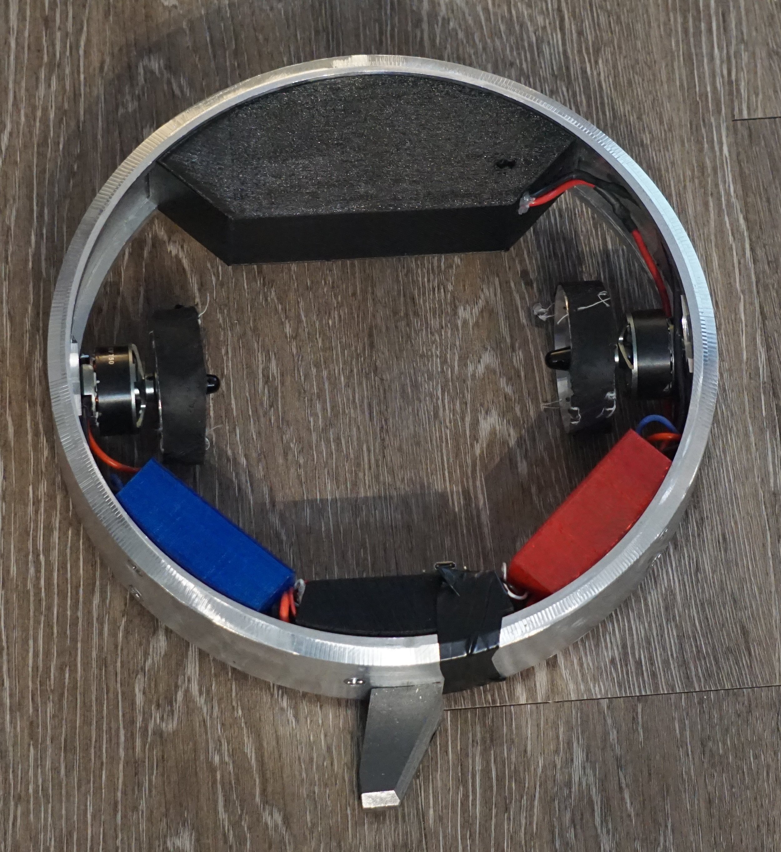
The BMM150 X and Y axis have a precision of 13 bits, and a resolution of 0.3uT per LSB. We expect a maximum of 50µT of earth field, plus between 10.84µT and 225000µT of field depending on the distance to the motor magnets. As an aside, the magnetometer clips at 1300µT, so that imposes a limit how close we can be to the motor. We will limit it to 1000µT, which is 13.5mm away from our motor magnets. These numbers are relevant to the motors in our 1lb and 3lb robots, and so should be re-considered for other robots.

What’s Important to our fixed point considerations is the 50µT earth field, which corresponds to 166LSBs. From simulation, I know that Goertzel’s can operate on as few as +/-5 LSBs. So it’s reasonable to drop our resolution from 13 bits to as low as 10 if needed. But in the end the three bits didn’t make or break anything, so I kept them.

int32_t sample = (int32_t) (mMag->getReading());
mSampleBuf[mSampleIndex] = sample;
mSampleIndex = (mSampleIndex+1) % SAMPLE_WINDOW_SIZE;

The samples are kept in a circular buffer, so we don’t have to spend time manually shifting old data every sample.

Windowing

After getting the sample, the next operation is a multiply with our pre-computed windowing coefficient. From simulation I confirmed that as few as 8 bits of precision are enough for windowing to work correctly, so I will use that here.

$$\textrm{Window Coeff i} = 0.54 - 0.46\cos(\frac{2\pi}{N} i)$$ $$\textrm{FP Window Coeff i} = \textrm{int}(0.5 + (\textrm{Window Coeff i})2^\textrm{bits})$$

Where, reminder, N=32 and bits=8. These coefficients should definitely be pre-computed. They can be applied to your raw data like so:

windowData[i] = rawData[i] * windowCoeff[i];

The result will have 8 bits of precision, meaning it’s still multiplied by $2^8$. We will maintain this precision into the following section.

Fixed-point Goertzel’s Algorithm

int64_t d1 = 0;
int64_t d2 = 0;
for(uint8_t i=0; i<SAMPLE_WINDOW_SIZE; i++) {
  int64_t coeffd1 = (GOERTZEL_COEFF*d1) >> FIXED_PRECISION;
  int64_t y = mWindowedBuf[i] + coeffd1 - d2;

  d2 = d1;
  d1 = y;
}
int64_t resultR = d1 - ((d2*GOERTZEL_COSW) >> FIXED_PRECISION);
int64_t resultI = (d2*GOERTZEL_SINW);//This result has 2X precision!

//RP2040 hard-ROM float functions
float resultR_f = fix642float(resultR, FIXED_PRECISION);
float resultI_f = fix642float(resultI, FIXED_PRECISION*2);
//We choose not to compute signal magnitude
float phase = atan2f(resultI_f, resultR_f);
int32_t phaseFixed = float2fix(phase, 16);
int16_t heading = (int16_t) ((180 * phaseFixed) / PI_FP16);
if(heading < 0) heading += 360;

mutex_enter_blocking(&mHeadingMutex);
mAccelAccumulator -= ACCUMULATION_THRESH;
mAbsoluteHeading = heading;
mutex_exit(&mHeadingMutex);
mHeadingValid = true;

Additions and subtractions must occur between two numbers of the same precision, so you can see me shifting out extra precision in a couple places.

Re-Window Old Data

Now that we’ve delivered out result, we can start looking forward to the next cycle. The main thing we can do ahead of time is re-windowing our sample buffer, now with each sample shifted a position. This lowers the latency from sample to result, which is generally a good thing for us.

for(uint8_t i=0; i<SAMPLE_WINDOW_SIZE-1; i++) {
  uint8_t bufIndex = (mSampleIndex+i) % SAMPLE_WINDOW_SIZE;
  mWindowedBuf[i] = mSampleBuf[bufIndex]*mWindowCoeffs[i];
}

Using the Result

It’s not enough to use the Goertzel result alone, because we will only get a new result every 30°. To reach single-degree precision, we will have to supplement with accelerometer data.

Fortunately, the accumulator corresponds with how far we have rotated since the last magnetometer fix. We can even use the same extrapolation math to reach maximum precision.

//This is intended to be run by core0
int16_t MeltyCompass::getHeading() {
    uint32_t predictedAccumulation = 
        (mAccumulatorRise*(time_us_32()-mLastAccelSampleTime)) /
        ACCEL_SAMPLE_PERIOD;

    mutex_enter_blocking(&mHeadingMutex);
    uint32_t totalAccumulation = mAccelAccumulator + predictedAccumulation;
    int16_t heading = mAbsoluteHeading;
    mutex_exit(&mHeadingMutex);
    int16_t predictedHeading = (DEG_PER_THRESH * totalAccumulation) / ACCUMULATION_THRESH;
    return heading + predictedHeading;
}

This function gets run by core0 on demand. Since we have two cores operating on the same data, a mutex is employed. This prevents the cores from stepping on each other, as otherwise core1 may overwrite this data at the same time core0 is trying to read it.

Magnetometers: a Possible Way Forward

On the last post I detailed all the ways we screwed up our magnetometer implementation. Here I’m going to talk about how we can make it better.

I knew from our previous analysis that low-pass filters couldn’t separate our signal out. But I suspected an FFT might.

Long explanation short, Fast Fourier Transforms can take a chunk of sampled data, and compute how much signal there is at various frequencies inside the data. Lets demonstrate.

Here is the signal I originally expected to see, as recreated in a simulation:

Ideal field strength plot

But as discussed in my previous post, the motor magnets add a lot of noise. Here’s what that probably looks like:

Simulation of motor noise

This looks pretty gnarly, and does resemble the plot of actual data from the previous post. The untrained eye might think it’s impossible to get our ideal signal out of this plot, but that’s not quite true. Here’s what we get when we take the FFT of this data:

FFT of the noisy data

In this simulation, the robot is spinning at 1500RPM or 25Hz. So we see a matching peak at 25Hz, that’s the signal we want. But the motor noise represents as a peak at 75Hz and 525Hz.

There is a third peak, but its frequency is too high to appear in this plot. We will generally only consider the first noise component anyways, as it is the strongest and hardest to separate.

Now, the thing about FFTs is that not only do they give you the magnitude of a frequency component, they can also give you the phase shift. And for us, the phase of that 25Hz signal is our heading measurement. So if we can take an FFT of our magnetometer data and find the first peak, we can get our heading measurement. How hard could it be!

Slowly Adding Reality

We have to consider that FFTs are very expensive (read: takes a lot CPU time), and we are running this on a relatively slow microcontroller. So we need to take some shortcuts to make our algorithm cheaper.

First, we will only computer over a narrow window of data. The fewer the samples, the less work you need to do to compute the FFT. The tradeoff is that you lose some resolution; instead of knowing your signal is at exactly 25Hz, you can only know that it’s somewhere between 24 and 26Hz, for example. But even at 32 samples we keep enough resolution to work with.

We will also reduce our sample rate to one our magnetometer can actually achieve. For the BMM150 that’s 300Hz.

More realistic FFT plot. Robot is spinning at 18Hz

Here you can see that resolution tradeoff in practice. That said, our signal of interest (SoI) is still easily discernible.

But Can we do it Cheaper?

The thing is, we don’t really care about the FFT results of any frequency that isn’t our SoI. If we knew in advance what frequency our SoI is, we could try to compete a partial FFT of just that bin.

Goertzel’s algorithm is exactly this. Pre-compute some parameters given your sample frequency and signal frequency, and you get an algorithm that can extremely efficiently find the magnitude and phase components of just your signal frequency.

Results of a Goertzel algorithm on simulated magnetometer data, constant speed

You can find my python Goertzel implementation here. I used these sims to generate all of the plots in this post.

I’m flippant about saying we have knowledge of our SoI’s frequency because the use of an accelerometer to measure rotation speed is already well understood. I don’t love adding a back a $10 chip (H3LIS331DL) that I spent years trying to replace. But it significantly reduces the computation requirements of our algorithm, and it’s also critical to counteract the effects of acceleration.

The Effects of Acceleration

A meltybrain spends most of its time in a match accelerating. If it’s at top speed, it should be getting busy smashing its opponent and accelerating again.

So lets adjust our sim to account for this and see how our algorithm performs.

Results from a naive Goertzel of accelerating data

Turns out it doesn’t do well at all. Here’s another view where I calculate the heading error across the sim.

Showing phase error over time for a naive Goertzel on accelerating data.

This occurs because our SoI no longer exists at one frequency. As the robot accelerates, it increases in frequency. Goertzel’s, and FFTs in general, calculate as if the components of a signal maintain the same frequency over the window of samples. If this isn’t true, you get artifacts that throw results off. Here’s what our FFT plot looks for this simulation.

FFT result of data with accelerating components

As you can see, there are now “phantom” signals all over the plot. These will disrupt the measurements of our real signals.

Resolving this problem requires us doing something a little weird.

Adaptive Sample Rate

We can lean on a unique advantage that we have to fix our acceleration problem. That being, an accelerometer that can provide us near real-time frequency measurements. The H3LIS331DL accelerometer can measure at 1KHz, roughly 3X the sample rate of our magnetometer. If our rotation speed is accelerating, we can see that immediately in the data. Additionally, the BMM150 can be triggered manually. More on that in a second.

Reminder: the Goertzel’s algorithm must be configured for a particular sample rate and target frequency. The way these parameters work, however, is if you double the target frequency and double the sample rate, Goertzel’s will give the same exact answer.

So if the accelerometer measures that the robot is spinning 5% faster, we can boost the magnetometer sample rate 5% to match. Doing so will ensure the Goertzel’s algorithm will continue giving good answers with exactly the same parameters.

We can think about this another way. By saying we are configuring Goertzel’s algorithm for a particular sample frequency, we are also saying we are configuring Goertzel’s for a particular sample period. As long as we ensure each sample represents the same percentage of a signal period, Goertzel’s will provide valid data.

We can lean on the accelerometer to predict how much of a signal period has elapsed since the last magnetometer measurement. If we are seeing a higher rotation speed, then we can predict that the signal period is elapsing faster. Every millisecond, we get a new accelerometer measurement that we can use to adjust our prediction. If we trigger a magnetometer measurement after exactly the correct amount of signal period every time, Goertzel’s will give us the correct data no matter how the frequency changes over the sample window.

Simulation of a Goertzel’s algorithm with adaptive sample rate, in a dramatically decelerating scenario

Pictured above shows our “adaptive sample rate” in action. The robot quickly decelerates to half speed, but Goertzel’s stays roughly on track throughout. It accomplishes this by slowing down the magnetometer samples to match the decrease in SoI frequency (you can see the X’s become increasingly spread out in the plot)

That simulation is also a bit more advanced, in that it includes the effect of measurement error. We are effectively doing a discrete time integral of the accelerometer data, after all. Any error present will add up to an extent. However, it will not add up infinitely over time like it would if were trying to get position directly from our speed measurements. In our case, the error effectively “resets” every measurement. This has been a lot of words, so below is a graph that attempts to demonstrate how our adaptive sample rate helps.

Showing how rotation speed can be integrated to correct for acceleration in the Goertzel/FFT data

As an aside, you might wonder how the heading measurement can be useful given that the sample window now represents a variable amount of time. Especially since the heading measurement is relative to the first measurement in the window, so all of our measurements are 32 samples late! The trick is, if we are ensuring that each sample is relatively the same period apart, then the entire window has a relatively fixed phase shift from the first sample. And as discussed in previous posts, fixed phase shifts can be ignored because they will be adjusted manually regardless.

Lets see how this algorithm performs.

Heading error of an adaptive goertzel implementation in a rapidly decelerating environment

If the worst our heading error gets is 20°, we’ll take it.

A Magnetometer Collides with Reality

So the magnetometer didn’t work.

The week of the competition, we were finally able to integrate the robots. I took a lovely working magnetometer, and spun it in a robot for the first time. What I got was useless noise, noting several revolutions per revolution.

As noted in my event report video, at the midnight hour we converted the magnetometer’s analog circuitry to read from an IR photodiode instead. This allowed us to at least compete

Most things don’t survive their first contact with reality, and we’re no exception. In this post I’m going break down exactly what went wrong, the steps we took to fix it, and where we ended up.

Motor Noise

There is also a particular noise component, but further testing indicated that it was introduced by the co-located brushed motor in my test rig. So I don’t expect it to be present in the arena.

- Spencer Allen, A Rotating Coil Magnetometer for Meltybrains

I was completely wrong about how much affect motor noise had. The bulk of my noise came from exactly this, my drive motor magnets were being picked up. Lets actually do some napkin math to investigate this.

Each drive motor has 14 magnets in the rotor. I don’t have an exact field measurement, but similarly sized magnets are rated at 0.225T, so we will use this. I originally discounted the effects of these magnets because of the distance from the coil, that being around 130mm center-to-center. According to this handy calculator from K&J Magnetics, we can expect a field strength of 10.84µT. As a reminder, we are expecting 50µT of earth field, so that doesn’t seem too bad. But the other thing to remember is the coil picks up changing fields, not static ones. The speed at which the field changes matters too.

The wheels are 2” diameter, and are 3” from the center of rotation.

$$p_\textrm{wheel} = \pi d = 159.6mm$$ $$p_\textrm{at wheel} = 2\pi r = 478.8mm$$ $$\textrm{Wheel turns per revolution} = \frac{p_\textrm{at wheel}}{p_\textrm{at wheel}} = 3$$

So for every revolution, the wheel turns three times.

To explain from here I’m referencing the paper “Filtering of Magnetic Noise Induced in Magnetometers by Motors of Micro-Rotary” [Unwin, 2015] They explain that brushless outrunner motors generate three categories of noise:

  1. Noise from the alternating magnet fields, at 14X the motor rotation speed

  2. Noise from uneven demagnetization of the magnets over time, at roughly 35X the motor rotation speed

  3. Noise from some magnets being stronger than others, at 1X the motor rotation speed.

The last bullet is bolded because it is the most dangerous to us. At only 3X the frequency of our signal of interest, it is nearly inseparable. To add injury to injury, the paper referenced above identifies this noise component as the strongest of the three.

Impact Analysis

In order to demonstrate the effect of this noise, lets run the numbers on source 2 from above. Source 2 is a little easier to calculate for, but keep in mind it’s not as a strongly interfering as source 3!

With 14 magnets in the rotor, the field changes 7 times per wheel turn. So in total the field change has a frequency 21 times the bot rotation speed. Lets plug these numbers into the equation from the previous part:

$$\varepsilon=-NAB_E\omega\cos(\theta)$$

$$\varepsilon=-(3000)(0.025m \cdot 0.038m)(0.00001084T)(157 \cdot 21 rad/s)\cos(42 \cdot \theta)$$

$$\varepsilon=-0.2037\cos(21*\theta)$$

Wowza, 200mV is 10X the signal strength of our actual signal! Though, slight wrinkle, it’s also at 42X the frequency of our actual signal. That makes the frequency $$25Hz \cdot 42Hz = 1050Hz$$, which is above the cutoff frequency of our filter. So to really understand what we’re up against, we need to evaluate the performance of our filter at that frequency.

Low Pass Filter Performance

According to our simulation, our filter attenuates by around 34.5dB at 1KHz, or 1 over 53. So On the output of our filter, our signal is 3.843mV in amplitude. That is ~5.7X smaller than our signal of interest, but still not great.

It’s also useful to evaluate at a different frequency, since our filter attenuation is logarithmic but our signal is linear. Lets take half the speed above, or 1250Hz

$$\varepsilon_{earth}=-(3000)(0.025m \cdot 0.038m)(0.00005T)(78.5 rad/s)\cos(\theta)$$

$$\varepsilon_{earth}=-0.011\cos(\theta)$$

$$\varepsilon_{magnet}=-(3000)(0.025m \cdot 0.038m)(0.00001084T)(78.5 \cdot 21 rad/s)\cos(21\theta)$$

$$\varepsilon_{magnet}=-0.0509\cos(21\theta)$$

The attenuation at 525Hz is roughly 26.5db, or one over 21.1.

$$V_{magnet}=-0.0024\cos(21\theta)$$

Sure enough, at this frequency, our noise component is now only 4.6 times less than our principle signal.

This is all pretty bad, so no wonder we were having trouble pulling the signal out. The noise is too close in frequency to be filtered, and it’s too strong to ignore.

Hard Consequences

As a result, the comparator was cut. There’s no way it could deal with the noise, no matter how much hysteresis was added. Instead, we attempted to sample analog voltages and filter it further digitally. This didn’t fare much better unfortunately.

Plot of raw magnetometer data

We gazed upon this plot, and despaired. We tried a couple filtering options, but in the end we were doomed. Realistically, we weren’t going to do much better than the analog filters. So this was the point we pivoted to the IR receiver.

The bright side here is that our analog front end could be easily re-purposed as a transimpedance filter for infrared. We got it running in record time.

Looking Forward

That all said, I wasn’t ready to give up on magnetometers.

I was recommended that paper after the event, and so could not benefit from it in time. It merely confirmed our experience, and definitively proved that simple filters weren’t going to work. With the strongest noise component only 3X the principle component, there’s basically only one technique that can separate them. More on that next time.

The other thing we learned is that while our rotating-coil magnetometer proved incredibly high-performance, this was ultimately wasted. It showed us in incredible detail how noisy we were, but math means that it didn’t make it any easier to pull out the signal we were looking for. At the same time, we identified a COTS magnetometer that had good enough specs. The BMM150 has sensitivity good for earth field sensing, and a sample rate well over Nyquist at 300Hz.

All that to say, goodby to the rotating-coil magnetometer. I learned a lot, it succeeded in its goal, but it’s too expensive for it’s worth.

Event Report: Robot Ruckus 2021

Robot Ruckus 2021 didn’t go very well. Let’s get that out of the way first.

And unfortunately I don’t really have enough footage to make a proper video, so I’m going to skip it for this competition. Sorry everyone! Instead I’ll try to sprinkle more media in here than I normally would.

I’m going to spend this post talking about what we did going into the event, what went wrong, and what we’re going to do going forward.

What we did different

CnC Manufacturing

Pierce now has access to a nice CnC machine, and this has upped our manufacturing game tremendously.

The Halo chassis, partially machined

With a CnC in hand, we can add more complex geometry to Halo’s chassis. We no long use wheel weights to balance the bot, instead adding material to the ring to ensure balance by design. Flats were added across from holes to make the holes easier to punch. And the need for motor mount plates was removed, we can bolt the motors directly to flats on the inside of the ring.

For Hit ‘N Spin it made a big difference. We now machine Hit ‘N Spin’s chassis out of UHMW blanks. This should prevent Hit ‘N Spin from exploding on contact like last time.

Hit ‘N Spin chassis being machined

Hit ‘N Spin not exploding

Halo Electronics Placement

I wanted to simplify the wire routing in Halo by moving the circuit board near the battery. My thought was the circuit card could double as power distribution, such that the ESCs route to dedicated pads for each. No more Y splices.

Here’s what we came up with:

This new placement saved a lot of weight, and made our “squishy bits” a smaller target.

After seeing Project Liftoff get taken out by Sawmuri, we invested in some better top and bottom armor for your battery box. Seen above, both sides have a UHMW/Nomex (fiberglass)/PLA sandwich to deal with a variety of incoming attacks.

Halo Electronics

A new board was spun for the new placement in the chassis, but no major changes were made. In fact, a lot of extra pads and unpopulated features had to be removed to make room (it was a layout nightmare).

Unified Codedbase

I spent a good amount of time combining Halo and Hit ‘N Spin into a single codebase. This ended up more than paying off, as any improvements in one automatically payed off to the other bot. I also took the time to completely remove ST’s HAL libraries, which I’ve been suspicious of from the beginning. Now all of the code that is running has been written and verified by me.

The Handheld Controller

To support a new experiment I’m working on, a new handheld controller was made from scratch. I’ll detail the experiment in a later post once I have it working, but I’ll briefly list the specs here:

  • Raspberry Pi 4 with Touchscreen Hat

  • Thumbstick and deadman’s switch

  • Xbee radio

  • Picamera module

  • USB power bank

The controller software was running off of a python application. The screen showed battery information and RPM, which was nice to have. But the touch screen wasn’t as reliable as a mechanical switch, and caused some problems during a Halo match.

What Went Wrong

Both bots had individual problems.

Hit ‘N Spin didn’t have traction

Going into RR2021 I had the highest hopes for Hit ‘N Spin. It seemed nigh indestructible, and it’s unusual geometry is hard to fight in antweights. But ultimately, it was defeated by the floor.

This is close to the floor used

Losing a match because of the floor seems like a right of passage in battlebots, and I can now say I lost a tournament because of it. They used a plastic backsplash panel as the floor for the tourney. It was enough grip to get spun up, so it took a lot of experimentation to figure out what was going on. Turns out, it was not enough grip to translate. Hit ‘N Spin spun up, then sat there until it got counted out.

Thankfully, Halo maintained enough traction to translate, but…

Halo had motor problems

The untimely discontinuation of our beloved AX-2810Q motors caused us to source a replacement model. The new motors were a rollercoaster. They boosted our acceleration and top speed appreciably, which was great to see. But two days before the event we realized they increased wheel wear dramatically.

And finally, when our first hit landed, the bearing in one of them exploded.

For the second match we were able to mount the old motor on instead, but incredibly that motor lost its bearing too!

Though even if the motors had held, there were issues in the battery box.

Fracture points circled in red

The battery box was cracking in multiple places, from the shock of impacts alone. It was still together by the end, but we knew it was only a matter of time before it exploded.

The impactor on Halo is about a half inch longer than the first revision. And it is much more fortified, such that it does not yield on impact. As a result, Halo hits way harder than it did at first, and its internals get shredded in the process.

We’re playing a game of finding the next weakest link. Eventually, we’ll find them all. Until then I expect us to continue losing more than we win!

What We’re Going to Do

Customized motors

Clearly stock motors aren’t cutting it. We need to replace the bearings at a minimum, but we’re looking to go further and convert the propdrive motors into hubmotors. This should hopefully put motor reliability issues to bed.

No more PLA

We used PLA for the battery box, because that’s the only thing our printers can do. We knew PLA was brittle, and used careful design to mitigate issues. I then hit a brick a couple times to double check.

But clearly in the heat of battle, PLA can’t handle the shock. It will be for prototyping only. We will be getting printed parts made professionally and mailed in from now on.

Figure out how to translate on “weak” floors

I suspect smarter motor control could have saved Hit ‘N Spin. So I plan to acquire the same flooring and get it to run reliably.

Driver Change

Pierce will be taking over driver responsibilities going forward. After so many events, we’ve agreed that I’m better at running the media side of things. When these bots are working they basically drive themselves, and Pierce has a ton of RC plane and drone experience, so we think he’ll do great.

As for me, I got an enormous amount of practice with my Chronos 1.4 during the event. I’m now at a point where I can reliably keep the action in focus, so it makes sense to have me do camera work full time.

Build a 30lb Hit ‘N Spin

Okay, this isn’t really a lesson learned. In fact, we probably shouldn’t. But it just sounds too fun, and we’ve got ideas we’ve been dying to put to the test. So we’ve started designing our next bot, which we’re calling “Bat out of Hell”. Hopefully we can get it together for this year’s Norwalk Havoc Season!

Chronos 1.4 Captures the Glory

To wrap up this post, here’s some footage I caught while we were sitting around being losers.

If anyone was at the event and I might have gotten footage of their bot, drop a contact form with a link to a bot photo and I’ll send you what I have.

Event Report: Bugglebots 2019

The footage is finally here! Bugglebots happened back in May, and the volunteers have been working in whatever time they could find to piece the footage together into a clean presentation worthy of television.

Fortunately, the first heat featured Halo!

As of writing, the whiteboard matches are the only things left to air. I will post the relevant footage when it arrives.

Bugglebots was overall a great time

What an event! We got to see some of the best bots in the sport, and meet some of the best builders in the sport. Everyone was friendly and excited, and even as things broke and people got eliminated, the other builders maintained their professionalism and enthusiasm.

A quick aside, us in the battlebot community are blessed to have some of the most gracious people I have ever met. If you’re a fellow builder reading this, don’t take it for granted!

The various bits of downtime we had gave us the chance to look at everyone’s bot. The other builders were more than willing to show off their construction methods, and there was idea exchange going every direction.

Halo was exciting

We drew a crowd when we were just in the test box! I’m sure part of this is the novelty of the design, which will wear off eventually. But even ignoring that, people seem to really like the energy of Halo’s matches and the cool-factor of the LEDs. Not to mention that people usually expect something to explode when it’s in the arena.

We even had a spectator stop us in the audience section to tell us that Halo was her favorite bot, which was a highlight of the event for us. Halo is a lot of work to develop, and if there wasn’t such a positive response from everyone I’m not sure we would still be working on it.

Halo Had Controls Issues

As of writing, I can only talk about things from heat 1. I will update with lessons learned when more footage appears.

But in heat 1, it’s pretty clear that something wasn’t right. In match one, we couldn’t get the beacon to connect. At the time, we thought it was simply a lack of power. The arena was bigger than we had ever fought in, so it made sense at the time. But later testing back in the states finally found the culprit: the polycarbonate.

The Problem All Along

Now, the polycarbonate sounds like an obvious issue. It’s in the way! But the beacon always worked fine while we solo tested in the arena, so for a long time we assumed that the polycarbonate had little effect.

That is, until Pierce set up a test rig. Using an infrared source, a light meter, and a small sheet of polycarbonate, he was able to demonstrate that the angle that the light strikes the polycarbonate at matters a lot.

This made a lot of things click for us. During events, when we did a test run in the arena alone, we typically stood right in front of the bot because there was no one in our way. This meant the angle of incidence was shallow, and the beacon worked fine.

But during matches, there is a ton of people crowding the arena. Us the driver, with our fancy beacon, gets confined to one spot. So when the bot inevitably bounced to a close corner, our beacon hit the polycarbonate at a steep angle and glared off. We couldn’t even try to move around to see if we could reach the bot.

In Maker Faire Orlando 2018 I first blamed the control issues on reflections. Now looking back, I can see that we lose beacon control when the polycarbonate is angled to us, and we gain it back when the IR has a dead-on path. Bugglebots was no different. The pit was adjacent to the wall we stood at. So when Halo bounced on top of the pit in match 2, suddenly the incidence angle went huge and we lost contact with the beacon. We were doomed by our untested assumptions.

Keep-Away Sticks: The Surprise Menace

“Those flimsy things? They’ll get peeled off on the first hit.”

Oh boy were we wrong. Rust-In-Pieces became the first bot(s?) ever to take Halo from full speed to pinned. Now, part of this was the excellent driving and the relentless recovery of the two bots. But the keep-away sticks made it much harder to land good hits and helped sap some energy before they rammed in. Had we known, we would have run Halo upside-down. This would have given the tooth enough clearance to avoid the sticks entirely and punch straight at the wheels.

Event Report: Robot Ruckus 2019

Robot Ruckus 2019

20191109_093841.jpg

We didn’t do as well in the rankings as we had hoped, but the event was still quite successful. We learned a lot about the good and bad of our bot concepts, and it made me feel really good about our bot concepts going forward.

Match Footage

What We Learned

Lets break down our performance at RR2019.

Halo

Halo had an overall record of 1-2. This is not great compared to last year, but it I’m not reading too far into it. The judges decision in match 3 was controversial, and I think with the things we learned we can start to develop Halo into a mature, ass-kicking bot.

The good

Halo, of course, was as destructive as ever. We fought mostly wedges in RR2019, and we were still able to immobilize most of them. I don’t see any issues with the maximum energy or weapon engagement.

Once Halo got spinning, it was basically unstoppable. Wedges get punted across the arena after contact, giving Halo time to spin up again. It’s really difficult to pin Halo once this starts happening. This forces a wedge bot into the defensive for the rest of the match.

Twice during RR2019, Halo lost a wheel, and was relatively unaffected. I even got it out of a corner on one wheel during the rumble. It goes to show that the fundamental concept of Halo lends a lot to its effectiveness.

The Bad

Self-Destruction

Halo has a habit of losing parts for the first couple matches. It’s kind of a game of wack-a-mole, every new record-setting hit means something new breaks. We’ve fixed things every time they’ve come up, but to be really successful in a competition it needs to not happen in the first place. Lets review what has broken and how we fixed it:

MFO 2018: Xbee + Teensy comes out of their sockets (fix: lock in with epoxy). Connectors shear off the board (fix: direct solder connections only). Aluminum frame cracks and bends (fix: new tooth geometry).

Bugglebots 2: <redacted>

Now for Robot Ruckus 2019, we have:

Radio header solder joint crack: the stencil method doesn’t deposit enough solder for these big headers. I need to solder this with an iron from now on.

Voltage regulator pin shear: looking at options here. Easy method is just add more epoxy, but I’m also looking at new regulator modules. For either option, more epoxy.

Controller mount crack: new print materials, new print direction (layer lines tangential to ring).

How do we fix it really?

Like I said, fixing spot issues isn’t good enough. We need to take a look a the root of all of this and see if we can prevent spot issues in the future.

20191110_112039.jpg

Epoxy is a common theme here. I think I need to bite the bullet and start potting the board, which basically means covering the entire board in epoxy. I’ve only done spot epoxy before, because once the board is potted you can’t repair any solder connections or replace any parts. But the electronics are mature enough that I think potting is a reasonable thing to do. Once potted, components shearing off should be a thing of the past.

It’s time to retire PLA as a building material. Our assumption was that it was fine for parts not seeing direct combat, but at this point every 3d printed part has cracked at some point or another. Moving forward, every Halo component must be printed out of something stronger.

Controls issues

Our new corner-mount beacon actually does an excellent job reaching the whole arena. For once, the reference lock wasn’t an issue.

Instead, the control issues at RR2019 were due to a lack of testing.

For instance, Halo worked great until it was flipped upside down. After that my left-right got reversed! There is no good reason for that to happen other than it not being tested enough. We only got Halo spinning a couple days before RR2019, and it really showed. I was finding edge cases in the control code during matches, which is unacceptable. It can be argued my driving mistakes early in my third match cost Halo the whole tournament.

How do we fix it really?

The real culprit is a lack of time before RR2019. Getting two bots ready was tougher than expected. We need to ensure we have more time to test before tournaments in the future, and perhaps that means pulling some bots out. I would rather have one great bot than two mediocre ones.

Hit ‘N Spin

Hit ‘N Spin had a record of 2-2. Not bad for a totally new robot concept!

The Good

Like Halo, Hit ‘N Spin struck fear in it’s opponents. You can catch an audible sigh of relief from our opponent after its fourth match!

The reason why is likely that it’s impossible to threaten the “squishy” parts, such as the wheel or electronics. The reach of the blade is just too far. On top of that, it has the “can’t be stopped” quality of Halo. After a hit, Hit ‘N Spin can spin back up before an opposing wedge can recoup. The only way to win against it is to survive until the end.

In terms of damage dealt, Hit ‘N Spin does not disappoint.

I was very worried about Hit ‘N Spin getting stuck. There are a lot of positions near corners where Hit ‘N Spin can’t spin up, guaranteeing a match loss. But in practice it maintains so much energy after hits that it always bounces back.

The spinup time is exceptional. The one opponent that box-rushed failed to reach us in time. What also helps is the chaotic nature of Hit ‘N Spin’s startup. It always translates pseudo-randomly while it comes up to speed, making it hard for a box rusher to line up correctly.

The Bad

Like Halo, Hit ‘N Spin is prone to self destructing, only worse. The plastic part sometimes sees direct contact (mostly against walls and floors). It also sees some constant strain, as the motor is bolted into the plastic.

As a result, Hit ‘N Spin lost two of it’s matches to the plastic giving out.

20191110_150415.jpg

How do we fix it?

PLA is right-out for Hit ‘N Spin. I still have faith in the general design of the bot, but I’m looking at Nylon or something carbon reinforced. The catch is I need to insert the titanium mid-print, which imposes restrictions on the printer I can use, but I have a couple ideas moving forward.

Miscellany

Our beloved AX-2810Q motors have been discontinued by the manufacturer. We are on the hunt for new ones, given we only have three spares left.

The handheld controller is due for a major redesign. I’ll have an entire post for that, stay tuned.

What next?

We will be at RR2020 for sure, but that’s a year away! Bugglebots 3 may not happen if the rumors are true, and I’m not sure we would go even if it did (a lot of hassle). So we’re on the lookout for another competition to attend. Given that flights out of Orlando are cheap, we’re looking anywhere in the US. Or in other words: have robot, will travel.

Hit N Spin

So here’s what happened

Say you get to know a guy, by say, building a terrifying blimp with him. Say he tells you he can get you a one-time deal: free 5mm titanium sheets, with free lasercutting thrown in. Just send him a DXF and he’ll make it happen. What would you do?

I know I would make a silly battlebot!

Antweight Meltybrain!

Antweight Meltybrain!

When I spoiled this on reddit, I got a few people saying “One wheel? How?”. The truth is: meltybrains only need one wheel to spin! Translation is achieved from the wheels spinning faster on one side of the rotation than the other, which can be done with any number of wheels.

Now, that’s not to say two wheels aren’t helpful. Two wheels means double the power. It means faster startup time, since no part of the bot has to be dragged on the ground. It means that you can drive the bot in standard arcade mode. And it means you can lose a wheel and still keep spinning.

But this is an antweight! Ain’t nobody got weight for two wheels.

Design Criteria

3D model view, with center of mass overlay

3D model view, with center of mass overlay

I started from “I want to make tombstone except just the spinning bits”. By going with one wheel, it would be easier to stay within weight, and it meant I could use common motors/wheels/esc’s with Halo (yay common spare parts piles!).

Of course, the challenge with a design like this is the electronics aren’t as well protected as in Halo. The safest place is the center of rotation, but anything sitting there contributes very little to rotational inertia (read: hitting power). I eventually settled on the counterweight/blade approach. The counterweight (electronics, wheel) is very dense, and the blade is relatively less-dense. This means the blade stretches further from the center of rotation than the counterweight does. The tip of the blade to the center of rotation is 183mm, as opposed to 108mm to the end of the wheel guard. Doing the math, an enemy bot has to make it 75mm into Hit ‘N Spin without striking the blade before the squishy electronics are threatened. I’ll take those odds!

Design Implementation

Yup. It’s titanium

Yup. It’s titanium

The blade is lasercut from some 5mm scrap titanium sheet. The design of the blade was the primary method I had to control the center of mass.

The Enclosure

The electronics box is printed around the titanium to save on fasteners and space. This is a fun trick with 3D printers; a carefully designed printed object can have things inserted during the print.

People usually insert bolts or bearings into an object rather than a giant titanium blade. But the concept works the same. The result is an enclosure that is totally captive to the titanium, without any fasteners at all.

The cost is that you can’t really have spare enclosures. It can only be printed on, which isn’t realistic at a competition. We’ll see how much of a problem this actually is at Robot Ruckus.

The motor bolts right into the plastic enclosure. Bolting into plastic isn’t my favorite thing to do, but hey, it’s an antweight. I didn’t have the weight or space for much else.

Spinup considerations

Spinning up is strange due to just having one wheel. At first I planned on having some kind of post or pad for the bot to spin around (hence the cutout around the center of mass).

In practice, I didn’t have to add anything. At rest, the bot touches the ground by the wheel and the end of the blade. When the bot starts spinning up, it rotates around the end of the blade. This is great, as it’s a longer lever arm (meaning more torque to spin up faster). After the bot gets some speed, the blade slips along the ground, and the bot starts rotating around the center of mass. Meanwhile, the centripetal acceleration pulls the blade up, making the wheel the only thing in contact with the ground.

The blade stays low to the ground, making Hit ‘N Spin a kind of undercutting spinner.

Pursuing this strategy lead to an unexpected design constraint: the enclosure must not touch the ground when resting on the blade. Otherwise the bot high-centers, holding the wheel uselessly off the ground. I had to iterate the enclosure several times to make sure I had enough ground clearance.

Electronics

I had to jam an ESC, circuit board (with radio), battery, breaker, fuse, and connecting wire into a tiny box. My strategy was to use the circuit board to integrate as much of that as I could.

The guts spilling out of an earlier version.

The guts spilling out of an earlier version.

The circuit board I came up with has a fingertech breaker and 15A SMD fuse soldered right on. It has the display leds on top and bottom, the IR reciever diode looking out one side, and solder holes for the battery wires and ESC wires. I kept the meltybrain electronics the same as Halo.

The beauty of a custom circuit board here is

1) Routing connections on a PCB is way easier, lighter, and more space efficient than using normal wire.

2) I can position all of the location-sensitive components extremely precisely. When the board is inserted, everything magically lines up.

3) By providing extra solder holes, I don’t need to splice or T any external wire. Every wire is point-to-point.

Sure, designing a PCB is a lot more work up-front. But wow does it save you effort when you go to put everything together.

Everything jammed in

Everything jammed in

The PCB Schematic

Can be found here. I kept it as simple as I could, as I didn’t have space or weight for any fancy experiments. There was one exception: I added a LIS3MDL 3-axis magnetometer.

Quick aside: magnetometer testing

I had to at least try it. Supposedly, you can measure the earth’s magnetic field to get an absolute direction reference.

But I’ve worked with magnetometers before, and I know the truth. They are horribly noisy, and prone to getting messed up by everything. Motor turns on? your measurement gets biased. Steel object comes close? Biased. Route a trace wrong on your circuit board? Noise.

I put a magnetometer on Hit ‘N Spin (U1), and recorded the readings while I slowly spun the bot by hand. The data was just too imprecise to be useful. Unless you’re an expert on the subject, I wouldn’t try this at home.

The Layout

Done in KiCad 5.0

Done in KiCad 5.0

It’s a four-layer PCB, signal-ground-3.3V-signal. I had it manufactured at OSHPark. Note the lack of mounting holes! I removed them after I realized it was impossible to tighten a bolt in, and the board was already held in pretty well by the battery and cover.

Software

The code can be found here: https://github.com/swallenhardware/MeltyHitNSpinV1_1

This is a pared-down fork of the Halo codebase. On a basic level, it runs the same. But I don’t have a POV text display, and I only have one motor to control. I also had to re-calibrate the accelerometer, the data from which is below:

Calibration data and best-fit

Calibration data and best-fit

From the data, it appears Hit ‘N Spin maxes out at ~1300RPM. That’s pretty good!

Test Video!

Expectations

With both a lower rotational inertia per lb and lower top speed, I don’t expect Hit ‘N Spin to be the brutal slugger Halo is. I’m expecting Hit ‘N Spin to put on a good show. It’s a silly looking robot, and it’s pretty chaotic to drive. If it ends up in the pit twice, I’ll be happy as long as it got cheers doing so.

DShot ESC's for Meltybrains

Hello all, as of writing I’m still hard at work on the Gen 2 electronics. As part of this, I’ve recently struggled getting a new ESC protocol to work. The internet desperately needs all of the info about it in one place, so here we go!

ESC Protocols - Quick Overview

Most ESC’s support communicating over several protocols. Start talking in one of them and the ESC will automatically figure it out and start accepting commands.

A quick list of the most common protocols:

  • Standard PWM, also known as servo control. A 1ms pulse is low, 2ms pulse is high.

  • OneShot125: A faster PWM protocol, 125us pulse is low, 250us pulse is high

  • MultiShot: the fastest PWM protocol used. 5us pulse is low, 25us pulse is high

  • DShot: a digital protocol. baud rates from 150Kb/s to 1200Kb/s

As quadcopters keep getting better, they are demanding faster update rates out of their ESC’s. The ESC hardware and software has been desperately keeping pace.

I mentioned in previous posts that the ESC’s we were using weren’t responsive enough for the meltybrain algorithm, and it limited our translation speed. It turns out that part of that is the protocol we used.

We were using standard PWM protocol, which limited our update rate to only 500Hz. The analog nature of the protocol also caused us trouble, with the ESC’s being more susceptible to noise.

We can now take advantage of faster protocols, with better noise tolerance. I’m going to focus on the one we ended up using.

DShot

We picked DShot for two reasons: speed and noise. Being a digital protocol, you wont have small inaccuracies or noise issues. If you command 50% throttle, the ESC will see 50% throttle. And you can find ESC’s that support up to 1200Kb baud, which is pretty fast!

A lot has been written about the basic details of DShot, like this excellent overview at blck.mn, so I wont get too in-depth here. I’ll instead focus on the practicalities of implementing a DShot controller.

The Basic Idea

DShot is a digital protocol with several rate options, ranging from 150,000 bits per second to 1,200,000 bits per second. It’s a packet based protocol, where each packet consists of 16 bits. The first 11 bits are the command code, ranging from 0 to 2047. The 12th bit marks whether telemetry is requested, which would be transmitted over a separate wire (we don’t use this in Halo, sorry if you’re looking for details here!). The final four bits are a checksum, which is used by the ESC to validate the packet.

The 16 bits are transmitted in 16 high pulses on the signal line, where the length of the pulse indicates whether it’s a one (75% duty cycle) or a zero (37% duty cycle).


The Details

A quick forward, this information I determined through testing an ESC I bought off amazon. I don’t have an official standard, and can’t guarantee accuracy in all cases. But, it’s information I wish I had starting out, so I hope it helps.

In standard mode, code 48 is the lowest throttle setting and code 2047 is the highest throttle setting, for a full range of 2000 throttle settings.

I was able to dig up the function of codes 0-47 in the source code for the betaflight controller. The full list:

//this typedef taken from src\main\drivers\pwm_output.h in the betaflight github page
typedef enum {
    DSHOT_CMD_MOTOR_STOP = 0,
    DSHOT_CMD_BEACON1,
    DSHOT_CMD_BEACON2,
    DSHOT_CMD_BEACON3,
    DSHOT_CMD_BEACON4,
    DSHOT_CMD_BEACON5,
    DSHOT_CMD_ESC_INFO, // V2 includes settings
    DSHOT_CMD_SPIN_DIRECTION_1,
    DSHOT_CMD_SPIN_DIRECTION_2,
    DSHOT_CMD_3D_MODE_OFF,
    DSHOT_CMD_3D_MODE_ON,
    DSHOT_CMD_SETTINGS_REQUEST, // Currently not implemented
    DSHOT_CMD_SAVE_SETTINGS,
    DSHOT_CMD_SPIN_DIRECTION_NORMAL = 20,
    DSHOT_CMD_SPIN_DIRECTION_REVERSED = 21,
    DSHOT_CMD_LED0_ON, // BLHeli32 only
    DSHOT_CMD_LED1_ON, // BLHeli32 only
    DSHOT_CMD_LED2_ON, // BLHeli32 only
    DSHOT_CMD_LED3_ON, // BLHeli32 only
    DSHOT_CMD_LED0_OFF, // BLHeli32 only
    DSHOT_CMD_LED1_OFF, // BLHeli32 only
    DSHOT_CMD_LED2_OFF, // BLHeli32 only
    DSHOT_CMD_LED3_OFF, // BLHeli32 only
    DSHOT_CMD_AUDIO_STREAM_MODE_ON_OFF = 30, // KISS audio Stream mode on/Off
    DSHOT_CMD_SILENT_MODE_ON_OFF = 31, // KISS silent Mode on/Off
    DSHOT_CMD_SIGNAL_LINE_TELEMETRY_DISABLE = 32,
    DSHOT_CMD_SIGNAL_LINE_CONTINUOUS_ERPM_TELEMETRY = 33,
    DSHOT_CMD_MAX = 47
} dshotCommands_e;

Note that not all codes are shown in the list. It’s possible that different vendors use different code mappings, or it’s possible for extra features to be present. But it’s likely most vendors want to be natively supported by Betaflight, so that code list will be fine for the average user.

I haven’t tested all of these codes yet, but what I know so far:

  • If you change any settings with DShot commands, you have to issue the save settings command for them to take effect

  • To change the spin direction, set 3D mode, or save settings you must enable the telemetry bit in the associated command packet, and you must issue the command 10 times in a row for the command to take effect.

  • If you issue command 0 and the ESC is not armed, it arms the ESCs with the throttle ranges set to <Either max range or the pre-programmed ranges, I haven’t worked out which>. If the ESC is armed it stops the motors. This command should be used if you want the motor to be stopped. If you try to use a throttle setting to stop the motor, it still spins slowly.

  • If you stop sending commands, the ESC disarms. I haven’t timed the required update rate, but it’s pretty fast (10ms or less). This is a good thing, I was worried for a time that my bot would keep spinning if the code crashed!

DShot Bidirectional Motion (3D Mode)

If you enable 3D mode, the throttle ranges split in two.

  • Direction 1) 48 is the slowest, 1047 is the fastest

  • Direction 2) 1049 is the slowest, 2047 is the fastest

  • 1048 does NOT stop the motor! Use command 0 for that.

Transmission Code

The goal with the code is to support the maximum data rate (1.2Mb) while using minimum CPU time. There are two general schemes used to talk DShot:

  • Use an SPI peripheral, and send three bits for every “bit”. sending a “100” is a “zero” and “110” is a “one”

We didn’t have an SPI port hooked up to our motor control pins, since we were originally expecting to use PWM to control them. So we chose option two:

  • Use a timer peripheral to send a PWM signal, and modify the duty cycle after every pulse

We needed to change the duty cycle 16 times over the period of the transmission. We could have programmed a loop that waits for the timer to send a pulse, and then load in the next duty cycle. But that would mean the code was stuck serving the transmission for the full duration, which would take too long.

Instead we used something called DMA, or Direct Memory Access. This is a fairly advanced microcontroller technique, but when used correctly it can make your code extremely efficient.

Our microcontroller (STM32F446) has a DMA peripheral that can be programmed to move a byte or a list of bytes from one location to another. Importantly, it can make this transfer at the behest of a different peripheral (such as our PWM timer), without involving the CPU at all.

We set up the DMA to target the beginning of a list of 17 values and the duty cycle register in the timer. The 17th value of the list is just zero, which keeps the output low after the final byte is transferred. Every time the timer is about to reset and transfer the next pulse, it issues a command to the DMA to transfer a single value. This updates the duty cycle for the next pulse. The DMA peripheral knows to only send 17 values, after which it will disable itself.

When we want to send another message, we just update the first 16 values with the new message, and re-enable the DMA peripheral. Below is my setup code for the timer and DMA. Again, this is for an STM32F446. I’m using ST’s HAL library for definitions.

    //make sure the end is set to 0
    //the last packet is 0 to make sure the line stays low when we aren't transmitting a code
    motorPulseTrain[16] = 0;

    //setup the timer
    timInst->CR1 &= 0xFFFE; //disable timer

    //disable the dma stream
    dmaStrInst->CR &= 0xFFFFFFFE;
    //wait until the stream is disabled
    while(dmaStrInst->CR & 0x00000001);

    timInst->CNT = 0; //clear counter

    timInst->DIER |= 0x0200; //enable DMA requests on CH1 (no interrupts enabled)
    //timInst->DIER = 0x0100;//send dma request on update
    timInst->CCMR1 |= 0x0010;//channel 1 active when the timer matches
    timInst->CCMR2 |= 0x6060;//channel 3 & 4 are active when timer < count
    timInst->CCER |= 0x1101;//output compare 1, 3 & 4 outputs are enabled

    timInst->ARR = DSHOT_PERIOD; //sets the frequency to the DSHOT baud rate

    //set the DMA trigger channels to fire right before the time rolls over
    timInst->CCR1 = DSHOT_PERIOD - 7;

    //setup the DMA on the peripheral side
    timInst->DCR |= 0x000F;//one transfer, starting from CCR3

    //setup the DMA peripheral
    dmaStrInst->CR = 0x0C032C40;//channel 6, very high priority, size 4 peripheral offset,
    //half word data sizes, memory increment, memory-to-peripheral

    dmaStrInst->M0AR = (uint32_t) motorPulseTrain;//set the peripheral address

    //enable the timer
    timInst->CR1 |= 0x0085; //enable timer, prescaler=1, auto-reload enabled

You also need to configure the appropriate GPIO pins for alternate function to make sure the capture-compare channels drive outputs.

When setting up a transmission, we first need to work out what bits we’re sending. Below is how we calculate the checksum and build the packet:

void issueDshotCommand(uint8_t motor, uint16_t command) {

    //compute the checksum. xor the three nibbles of the speed + the telemetry bit (not used here)
    uint16_t checksum = 0;
    uint16_t checksum_data = command << 1;
    for(uint8_t i=0; i < 3; i++) {
        checksum ^= checksum_data;
        checksum_data >>= 4;
    }
    checksum &= 0x000F;//we only use the least-significant four bits as checksum
    uint16_t dshot_frame = (command << 5) | checksum; //add in the checksum bits to the least-four-significant bits

Now that we have the command in binary form, we just need to turn it into an array of duty cycles. The exact timing depends on the baud rate you’ve chosen, but DSHOT_1_TIME should be 75% of a full period and DSHOT_0_TIME should be 37% of a full period.

    //wait until the stream is disabled
    while(dmaStrInst->CR & 0x00000001);

    //Convert the bits to pulse lengths, then write the pulse lengths into the buffer
    for(int i=0; i<16; i++) {
        motorPulseTrain[i] = dshot_frame & 0x8000 ? DSHOT_1_TIME : DSHOT_0_TIME;
        dshot_frame <<= 1;
    }

And finally we point the DMA at the channel for the motor we want to command, and enable the peripheral.

    //set the peripheral address to the correct channel
    if(motor == MOTOR1) {
        dmaStrInst->PAR = (uint32_t) &(timInst->CCR3);
    }
    else if(motor == MOTOR2) {
        dmaStrInst->PAR = (uint32_t) &(timInst->CCR4);
    } else {
        return;//if the motor selection is invalid, just give up
    }

    //start the dma transfer
    dmaInst->HIFCR = 0x0F7D0F7D;//clear all of the flags because I'm lazy
    dmaInst->LIFCR = 0x0F7D0F7D;
    dmaStrInst->NDTR = 17;//set transfer size to 17 bytes
    dmaStrInst->CR |= 0x00000001;//enable the dma stream

}


And that’s it! the DMA will happily chug along, push out our bits, and disable itself. It needs no further code interaction.

Halo Pt. 11: Mechanics of a Good Impactor [Guest Starring]

Hello Everyone! Today’s installment of Spencer’s blog is being written by Halo’s second part, Pierce! I’m the brains behind the mechanical design and implementation of Halo, along with sanity checking all of Spencer’s work. I wanted to write this blog post to discuss the weakest point of the bot from the previous competition: The ring.

The Ring

The chassis of Halo is a unibody construction of 6061-T6 aluminum. We started with a 10” diameter by 1/2” wall aluminum tube that I turned down on my work’s manual lathe. I machined it into a C profile to help reduce the weight. The thickness of the wall is just over 1/8 of an inch thick. We discovered that we were overweight on the initial turning, so I reduced the weight of the ring by approximately 0.25 pounds by adding a 1/4” chamfer at the edges of the bot. This reduced the overall weight of the ring to just under 1 pound. The chamfer is not ideal because it pushes wedges underneath us, but the rapidly approaching impactor helps knock away our problems.

Because of the thin nature of the ring, it introduces us to some structural problems.

The First Impactor

Our first design worked surprisingly well. The first tooth was just a small chunk of 1/2” A36 steel plate that had been trimmed down to save some weight. It was secured to the ring by two grade 5 1/4"-20 hex head bolts. I was immediately worried that the bolts may rip their way through the ring, or crack it in half. Needless to say, I was flabbergasted when the ring survived all the way through the competition. By the end of the competition though, it was cracking right at the base of the impactor.

The ring at the base of the impactor showing deflection and cracking

Now, why was this happening? It couldn’t be because we were slamming into things at 1100 RPM, that’s totally not what would happen…. Okay, I’m joking. The impact force that we are applying every time we smack into something transfers a very large load to the bot. How large of a load? Well, it really depends on multiple factors, mainly how much energy is transferred to the surface we are impacting and the time that the impact lasts for. I decided to do a simple A-B comparison of the strength of the old tooth to the new tooth, so I decided to call the impact load 100 times the weight of the robot, or 300 pounds. I figured that amount should show us some good results on the FEA simulation. You may have heard of the term FEA (or Finite Element Analysis) thrown around. It is a method of simulating the stresses on CAD parts. Most professional CAD packages have some method of doing FEA stress analysis built in. I simplified the model down to a small cross section of the ring with the original tooth. Simplification keeps the simulation run times short and reduces the likelihood that something weird happens. The ends of the ring become our “fixed points” for the FEA simulation, and the tooth is bonded to the ring in this simple simulation (I use a better contact set for the redesign, don’t worry).

Simplified FEA Model for the First Impactor

Simplified FEA Model for the First Impactor

Once all of the materials are defined, and I ran the simulation, I got results that I expected. The ring showed stress concentrations right around the tooth, with the ring deforming into the S-shape which is slightly visible in the after competition image above.

Original Tooth FEA with Von Mises Stress

Original Tooth FEA with Von Mises Stress

Okay, but what does this actually mean for our impacts? How close are we to actually causing damage to the ring? For that, I switched into the Factor of Safety (FOS) view. This shows how close each piece is to experiencing plastic deformation (the technical term for when something actually stays bent). The view is effectively dividing the shown stress by the yield strength. An FOS of 1 means that the material will survive if everything in the model is exactly correct with no simulation inaccuracies. Obviously, we don’t want that to happen, so we want a FOS that is higher than 1. An FOS which is lower than 1 is usually extremely bad because the part will deform under the load! What is a good FOS to target? That is really up to you. If you were selling parts for aircrafts or cranes or personal safety, the FOS’s are usually well defined by regulations. I like to keep parts on the higher end of FOS, usually 3 or higher, because they can stand up to greater hits. As combat robotics are one-off devices rather than mass-manufactured devices, having extra material costs / weight is not too big of an issue.

FEA FOS Plot for the Original Tooth Showing the Front.

FEA FOS Plot for the Original Tooth Showing the Front.

Whoa! The minimum factor of safety on the tooth is 0.29? Could that actually be correct? In fact, it is. If you look very carefully at the root of the impactor in the after competition image , you can see where the curve of the tooth actually curves slightly away from the ring (it’s right at the top right corner of the tooth in the image). It’s pretty hard to see in that image, but is more visible in person. So, we actually caught some plastic deformation there, but what about in other spots? What caused the cracking?

Original Tooth FEA FOS showing the Back of the Ring

Original Tooth FEA FOS showing the Back of the Ring

0.93? That’s under an FOS of 1, and we can see in the post competition image that the ring does bend and crack right in that area. I’d call this simulation close enough to use for an A-B comparison between the newer versions and the original.

Iterate, Iterate, Iterate Again

Now that I know why the ring is cracking, I set out to stop that from happening. I knew immediately that there were a couple ways to increase the strength of the ring.

  1. Change Ring Material: Not Feasible. Nobody makes 10” titanium tubing, and I really don’t want to turn down that big of a billet of titanium.

  2. Change Ring Thickness: Probably Not Feasible. We were close to the weight limit, and changing the thickness of the ring really increases the weight.

  3. Change the Tooth: The best option. We can redesign the tooth to reduce the stress that gets transferred to the ring, indirectly increasing the strength of the ring.

The ring was killed by the moment around the base of the tooth. That linear force of the impact was transferred as a bending moment to the ring. The short base of the tooth was causing a large moment on the ring. If I can increase the length of the base, I can reduce the moment on the ring, which should help prevent it from being damaged.

Iteration 1: The Thin Tooth

1st Iteration: The Thin Tooth

1st Iteration: The Thin Tooth

I started by just directly adding length to the tooth base. This put me far overweight, so I started trimming weight by decking the active area of the tooth to a 1/4 inch and adding some speed holes. I thought this design looked rather odd, so I decided to think about where I could actually remove weight in this part.

Luckily, there is software for that. I used another FEA tool called an optimizer to tell me exactly how much material I needed to have. You define the forces on your part and any fixed geometry that you want, and it tells you what you can cut off. Quantum from Team Robo Challenge is doing something similar.

Or, at least, that is the theory. I use it mainly to tell me which areas I can remove weight from safely. I never take the optimizer fully seriously, as if your assumptions are incorrect, the parts will be too weak. It truly is a garbage in, garbage out system. By feeding in the basic model of the iteration one tooth into the optimizer, it resulted in Iteration 2.

Iteration 2: The Hollow Tooth

I screwed up when I started this tooth. I forgot the critical rule of write ups. If you are going to write something up about this process later, make sure you document as you go, not after. I forgot to to take an image of the optimized part, and I used the optimized model to make the model, which overwrote the optimized model. If I go back to take an image, I have to revert all of my work… Thus, all you get is a description of what it looked like when it was fully optimized.

Iteration 2: The Hollow Tooth

Iteration 2: The Hollow Tooth

The optimizer spat out a model that looked close to this shape, but had rounded all of the edges to make them more like cylinders. The optimizer did this to reduce the weight, as those edges don’t add too much to the strength of the part, but do increase the weight. I kept them in the final model as I wanted to insure that the tooth would be strong enough. The actual reason why I removed them is that I can’t manufacture them. I don’t have access to a CNC mill, so keeping everything as nice straight lines makes it easier for me to make.

This setup was nice, but it did have a smaller base. What happens if I flip the (not visible) mounting hole on the right side of the image to the other side of the tooth to increase the base further?

Iteration 3: The Flipped Bolt

Flipping the bolt hole was a good decision. Adding that flip increased the base by almost an inch, which increased the strength of the ring. This is the iteration that we will be fighting with, so I’ll go into more details with this one.

Third Iteration: Hollow and Flipped Bolt Hole

Third Iteration: Hollow and Flipped Bolt Hole

Why does the arm that hangs off the back work? The best analogy that I can create is someone shoving you. If you are standing with your feet together, and someone gives you a good shove, you will probably fall over. The base provided by your feet together is too small. If you stand with your feet as far apart as they can go and you get a shove, one foot pushes harder down into the ground, while your other foot starts to lift. This is a similar concept to how the arm works. As the impact comes in from the right, the bending moment that gets applied is spread out over a larger area, reducing the overall force on the ring.

I setup the FEA with this model, and ran it.

Third Iteration FEA Showing a Gap between the tooth and the root.

Remember how I said that I was planning on using a better contact set in the future? This is where it starts. If you look at the simulation results above, you can just barely make out a gap between the tooth and the ring. This is a good thing. Why? The connection between the ring and the tooth is a bolted connection, which behaves similarly to stapling two papers together. If I staple two pieces of paper together, I can still peel the pieces of paper apart, but they won’t slide past each other. The staple analogy behaves pretty close to a simple bolted connection. I used a “separation, no sliding” contact between the ring and the tooth to ensure that the faces could separate, but wouldn’t slide. I then “bonded” the bolt holes together to simulate the bolt holding those faces together. Using the bonding contact does introduce some problems in.

Third Iteration FEA FOS

Third Iteration FEA FOS

The minimum factor of safety on this design is actually extremely small. It’s 0.29, and occurs right at the intersection of the bolt holes. This is a simulation artifact that I am choosing to ignore. Sharp corners near bonded faces usually end up getting large stresses shown, because the faces are perfectly bonded together in the simulation. This causes the math to freak out.

As can be seen, the factor of safety on the ring right at the base is now 6, in comparison to the meager 0.93 that it was in the previous model. The force on the tooth is the same. The pure blue that is shown is the maximum factor of safety shown. In actuality, most of the FOS is over 40 because the stress on the ring is so low in most locations. With an FOS that high, the lower end in the 1 to 5 range becomes really compressed, so everything looks red. I shrunk the scale down to make it easier to see what was going on, as seeing a super high FOS is not that useful.

With hollowing out the tooth, this tooth is 0.253 pounds, in comparison to the previous tooth’s 0.209 pounds. Not bad for only increasing the mass of the tooth by 0.05 pounds and getting a six-times strength increase.

Iteration 3+: I’m Not Quite Done Yet

I can’t leave anything alone. I just have to improve on that tooth design. Overall, there are some weight savings that are occurring on Halo. We wanted to be able to target 3 pound and 1.5 kg competitions, but that leaves us with some mass available to play with. Well, what does that mean for this design? The answer: bigger and badder teeth. Meet iterations 3+ and 3++.

Halo Third Tooth Iterations

Halo Third Tooth Iterations

Each tooth is respectively 0.253, 0.330, and 0.451 pounds. I’m hoping that I can use the largest tooth because that results in the largest bite and available kinetic energy. If either of the larger teeth are too heavy, we can also grind down the fang at the end to reduce the weight into spec. Other than that, they are all identical, so we can swap in any tooth to meet weight.

Do these teeth work? I’ll leave that for you to decide. Here are the FEA results for the large tooth.

Halo Third Iteration FEA Large Tooth.PNG

Even with the largest tooth, we still get a factor of safety of safety of 3 with a 300 pound load at the end of the tooth. That should hopefully allow us to last a full competition without the ring cracking.

The result: a pretty terrifying set of numbers.

  • Overall Bot Radius: 7.75 inches

  • Ring Radius: 5 inches

  • Resulting Bite: 2.75 inches (35% of total radius)

  • Top Speed: 1100 RPM

  • Tip Speed: 75 fps (50 MPH)

  • Total Energy Stored @ 1100 RPM: 250 Joules

Meet Halo V2. Terrifying, even for us.

Halo Pt. 10: After Event Report

I just took Halo to its first event, Maker Faire Orlando 2018. The bot performed great, laying down hit after brutal hit, and eventually took second place. You can find all of the match footage below:

I’m going to take this post as an opportunity to summarize the good parts and bad parts in greater detail.

The good

Halo laid down punishment

It’s clear that halo could transfer energy. We were spinning slower than planned, but the improve rotational inertia made up for the lost energy. And the low speed and large weapon gave us enormous bite potential.

Halo took punishment

Even if most of that punishment came from itself, it’s still clear that the monobody design made for a tough bot. I still need to see what a good horizontal spinner would do to us, but the vertical spinners weren’t able to do much to the chassis. There just weren’t any good surfaces to attack.

The motors also proved tougher than I had originally thought. We didn’t have to replace a single one all competition, despite the direct-driven wheels.

Halo was tactically difficult to attack

We could attack in every direction at the same time. This was especially perilous for other spinners, which may not be designed to withstand powerful hits. Against wedge bots, we packed so much energy that even a successful deflection knocked our opponent away. This allowed us to spin back up in between contacts, preventing the wedge bot from pinning us.

Halo looked good

Battlebots is at least 50% showing off, and the LED display made a great show. The pinball action also made for a kinetic, exciting match.

The bad

The beacon has multipath issues

The sensor-fusion system detailed in this blog is great at filtering out spurious reflections, but what we saw in the match were consistent reflections. The result was that the beacon locked on to a random direction. I eventually got used to it and was able to adjust my driving, but it’s clearly not what was intended.

The tooth warps and cracks the chassis around it

Amazingly, the aluminum ring yielded before anything else did. It’s a testament to Pierce’s design and machining ability that it warped in this way, and still laid down punishment. Still, we should shore up the chassis there to prevent this from happening again.

The electrical components were not shock-proof enough

I need to more careful with my component selection and mounting strategies. More epoxy is also good.

The LEDs don’t have the best viewing angle

The LEDs are partially obscured by the modules on the circuit board, and It’s not always easy to see inside the ring. It would be better to find a way to make them shine outwards.

So what’s next?

We feel really good about this design, and other people seem to enjoy it too. So we will continue competing with it.

Of course, we still have a lot of work ahead of us. The ring is a total wash. even though it “survived”, the crack in the chassis would only continue to get worse. The circuit board took too much damage, and would need to be replaced even if we weren’t marking any changes. On top of this, we are looking at some big design changes.

We are changing the absolute reference sensor

I’m not going to remove the infrared beacon entirely. it barely takes any board space or processing power, so we might as well keep it as a backup. I’m currently investigating other methods that can provide an absolute reference, which if feasible will be detailed here.

There also may be a way to make the beacon better. If I offload some extra processing to the microcontroller, I can look for the strongest signal instead of just the first signal. This may be able to ignore reflections entirely.

We are changing the processor

The teensy served us well, but for mechanical shock reasons we should keep the number of plug-in modules to a minimum. I’m currently looking at the STM32 line as a replacement. Regardless of the choice, we will also port the code from arduino to straight C.

We are changing the ESC

The ESC’s we had were wonderful for what they were. They proved robust and powerful. However, if I tried to change the motor speed too much too fast, they would lose track of the motor and reset. This limited how fast I could translate.

I think the best thing to do is add sensors to the motors. This will give me much better control over the motor, improve spin up times, and let me win pushing matches.

The motors will stay the same, I can just add sensors to the outside of the case. But the ESC will have to support sensored operation. So goodbye ReadyToSky 40A.

We are changing the LEDs slightly

I’m investigating ways to make the LEDs shine outwards. I would also like to take advantage of a faster processor and go from five LEDs to seven. This will let me show more detailed images.

Halo Pt. 9: Accelerometer Calibration

In this post, I'm going to talk about how I calibrated the accelerometer in my bot. The calibration finds the relationship between measured acceleration and robot speed.

Some definitions

Measured acceleration comes into the processor in units of "LSB", or least significant bits. It's a jargon-y term that basically means raw data. We can convert LSB to g's by finding how many LSB are in the full-scale range of the accelerometer, then dividing by the full scale. But it's an unnecessary step since in the end we don't care about g's. We're going to directly relate LSB to robot speed.

As discussed in the previous post, we are expressing speed in terms of microseconds per degree to allow for more integer math. Here is what our angle calculation looks like:

code_new.PNG

Where robotPeriod is our measurement, in microseconds per degree.  The purpose of this calibration is to find the relationship between accelerometer LSBs and microseconds per degree.

The calibration method

We will define the relationship between accelerometer data and microseconds per degree by taking twin measurements from a real-world test. I use the test stand from part 6 to hold the bot, and then I slowly spin up and down the bot.

Meanwhile, the bot is measuring accelerometer data and beacon edge times. Beacon edge times tell us pretty directly our microseconds/degree, since they are measured in microseconds and we know our edges are 360 degrees apart. If you don't have a beacon on your bot, you can substitute with an optical tachometer.

Our bot decomposes the data and sends it to the controller (this is why we used XBee's as our radios).

robotPeriod in this case represents our raw accelerometer measurement

robotPeriod in this case represents our raw accelerometer measurement

On the controller side, we recompose the data, and send it to my computer over the usb cable.

data_receive.PNG

You can also do this by having a third XBee plugged into your computer via an XBee explorer, I just didn't happen to have one lying around.

On the host computer, I have a python script running that pulls in the data. It doesn't do much but put it into a file for later. 

writeToFile.PNG

I spun the bot up and down a couple times, and then shut down the test. Next, I wrote another python script to parse the data. Here are the points I gathered:

dataplot.png

As you can see, there are some good curves, but lots of artifacts! We will filter those artifacts out here. In the final code, the accelerometer and the beacon will work together to filter those out in real time.

Some easy artifacts to filter out include the ones at y=0 (when the accelerometer is reporting data but the beacon isn’t) and the ones at y= very large (which happens when the beacon misses several rotations. We add a simple high and low cutoff to filter those.

dataplot_artifacts1.png

Now we see the relationship we are looking for much more clearly. But, it’s in triplicate here. Every duplicate is due to the beacon missing N rotations. If the beacon missed every other edge, the us/deg would be double. If it missed twice in a row, triple, and so on.

We need to remove the duplicate curves, as they aren’t useful to us. To do this, we will use a piecewise linear cutoff.

The last artifact is the little “wing” at y=400. This one actually stumps me, I don’t know where it’s from. We’ll add an extra filter and move on…

dataplot_final.png

That looks much better. We need to use curve fitting to find the closest equation to represent this curve. Luckily, python can do that too!

curve_fit.PNG
finalplot.png

That looks pretty good! Lets take a look at the coefficients it gave us:

coefficients.PNG

This makes our equation:

equation.PNG

Ouch, that is pretty ugly. Luckily it only needs to run every time we get a new accelerometer measurement. And if it ends up being too slow in the future, we can use a lookup table instead.

Here is how the bot performs with the above equation and the improved accelerometer algorithm:

Halo Pt. 8: Improved Accelerometer Algorithm

Like the beacon in the post before, the accelerometer algorithm has some room to improve. The primary reason is the same as well: acceleration causes problems. And now, for the driest heading I have yet written on this blog:

What the algorithm does, in graphs

Like the improved beacon algorithm, there's really no better way to explain than with graphs. Here's what our bot is doing when it's spinning at a constant speed:

steadyState.PNG

Revisiting our first-order algorithm for calculating our heading:

linearAlgorithm.PNG

If we multiply the speed of the bot by how long it has been spinning that fast, we get how far it has spun. This is accurate so long as we are measuring infinitely fast, or so long as the robot continues spinning at the same speed.

Lets look at what happens when the robot accelerates:

accelerating.png

This case causes our algorithm to generate lots of error. It's not obvious where the error comes from, so lets visualize what our algorithm is calculating:

acceleratingBlocks.png

The red shaded area above is comprised of three rectangles, one for each measurement. It's width is the distance in time, it's height is the measured speed. What our algorithm tries to do is calculate the size of the area under the velocity line. This area equates to the distance traveled.

The simplest algorithm uses rectangles because they are easy to calculate area for (It's also known as the Riemann Sum). You simply multiply length (measured velocity) by width (time interval). But the graph above shows that when the velocity changes over time, some area is missed by the rectangles. All missed area represents error in the measurement, which causes drift.

If we want to reduce the error in our measurement, we can do two things:

1. Measure faster

If we measure infinitely fast, there will be no error. Or for a more likely solution:

2. Change how we calculate area

Instead of using rectangles, we can use a different shape that better matches our line. In the case above, the best match is a trapezoid, so we will use the trapezoidal rule here. The area of a trapezoid can be found with:

trapezoidBase.PNG

Where our trapezoid is defined as:

Trapezoid.png

The final equation, part A:

trapezoidalMelty.PNG

Given that you run this equation every time you get a new accelerometer measurement, the variables marked "i" are from the previous measurement and the variables marked "f" are from the recent measurement.

However, this equation can only run every time we get a new accelerometer measurement. If our code runs faster than our accelerometer (which is likely), then we will need to guess at our rotational velocity in between measurements. We can do this by borrowing an equation from the beacon algorithm:

linearExtrapolation.PNG

Remember this one? We can use it to extrapolate our current velocity given that we remember our last two measurements. Substituting in our variables:

The final equation, part B:

trapezoidalPredicted.PNG

Where (ω_1, t_1) is the earliest measurement, (ω_2, t_2) is the most recent measurement, Θ_2 is the angle at the most recent measurement, t_f is the current time, and Θ_predicted is where we expect the bot is pointing now.

Practical Considerations

In my implementation, I wasn't able to use the equations above as-is. This is due to the limitations of embedded arithmetic.

Time in my bot is measured in microseconds, but distance is measured in degrees. so to bridge the gap, my velocity term needed to be in units of degrees per microsecond. In practice, that is a tiny number. A speed of one revolution per second is 0.00036 degrees per microsecond!

Our microcontroller doesn't have a floating point unit, so any floating point operations are emulated in software. Consequently, floating point operations will be very slow. To remedy this, we can try to minimize our use of floating point in favor of integer math.

Instead of running calculations using degrees per microsecond, we can use microseconds per degree. This turns our 0.00036 into 2777.78, which (rounded to 2777) is much faster to do math with.

To support using inverse speed, however, we need to change our equations.

invertedOmega.PNG

This doesn't help much on it's own, but we can move the equation around a bit

finalInverted.PNG

To explain why this equation works better, lets say that the robot is moving at a constant 1000 rpm (around where we expect to operate) and the accelerometer is being sampled at 100Hz.

1000 rpm equates to 166.67 us per deg, which as an integer rounds down to 166. This is tau.

t_f - t_i is the time between measurements in microseconds. At 100Hz, that time is 10ms, or 10,000us. 10000/166 = 60.2 degrees.

I was able to do all of this math with integers only without losing too much precision. That would be impossible without redefining the equation in this way. This method can be used for final equations part A and B similarly.

Conclusions and Caveats

These equations should present much less drift than previously. Like for the beacon algorithm, we can trade complexity for precision.

The main caveat here is that error is still generated whenever the acceleration changes. This should not cause as much of an effect as acceleration did on the rectangular method. But if you truly want the best-of-the-best here, you can substitute the trapezoidal method with Simpson's rule to account for when the acceleration varies over time.

And you're only going to be as accurate as your calibration. See my next post for how I calibrated my bot.

Thanks to teammate Novia Berriel for working out the math

Halo Pt. 7: Improved Beacon Algorithm

In my last post, I introduced two sets of algorithms. One to run a beacon-only system, the other an accelerometer system. The algorithms were fairly easy to work out the math for, and fairly easy to express in code.

But say you need better. Say you need a perfect flicker display, or the easiest-to-control meltybrain bot possible. If you're that kind of builder (I am, at least), then you're in luck. We can take these algorithms a step further. The math is harder (read: longer), so I'm splitting this up into a post for both sensing systems.

Beacon Sensing, part 2

In the previous post, I showed graphs with beautiful, straight lines. The original algorithm works great if this is the case. But what if it's not the case? What if, for instance, the bot is accelerating?

linearBeaconProblem.png

As you can see, the prediction diverges from reality. Our algorithm expects a line,  but the robot is accelerating. We get a parabola instead. The error resets at every measurement, so this may not be an enough of an issue for the typical meltybrain. But if you made it past the first paragraph of this post it must be an issue for you.

What if instead of keeping track of the last two edges, we keep track of the last three?

parabolic1.png

If we assume that all three points are on the same parabola, we can calculate the equation of the parabola and use it to find where we are now. The parabola equation is:

parabola.PNG

The equation has three constants we need to solve for. Fortunately we have three prior points to help us do that: (x1, y1), (x2, y2), and (x3, y3), where x1 is earlier and x3 is later.

parabolaEquations.PNG

Represented in matrix form:

parabolicMatrix.PNG

Solving for a,b,c:

solvedPArabolic.PNG

We can simplify by understanding that y1=-720, y2=-360, and y3=0.

simplifiedParabolic.PNG

Now lets pull the common "d" parameter off and substitute in more appropriate variables:

The Final Equations:

finalParabolic.PNG

Where t1-t3 are the measurement times (t1 being earliest), t is the current time, and Θ is the calculated angle. a, b, c, d only need to be recalculated at every beacon edge. Θ is calculated on every iteration. Here's what our graph looks like now:

parabolic2.png

These equations should work even if the bot is not accelerating. There will still be error in your calculation if your acceleration varies over time, but those events tend not to last very long.

An additional gotcha you should know about with either beacon algorithms (linear or parabolic) is that missed beacon edges can severely disturb your predictions. The bot will think it's spinning much slower since the edges it saw were so far apart. This disturbance lasts longer in the parabolic algorithm since the "memory" of the event lasts an additional 360º. Clever code can handle missed triggers, but it will need to be specifically coded in.

Thanks to teammate Novia Berriel for working out the math

Halo Pt. 6: The Code

You can find the full code here. Read on for a discussion on how it works!

I had originally planned testing controls code with the robot on it's own two wheels. But after a catastrophic failure in one of said wheels, it was determined I would need to wait for my partner to machine some new ones out of aluminum. That would take too long, so I picked up some clamps and printed a test stand.

testSetup.JPG

Test stand in place, I started working on the code in earnest.

codeBlockDiagram.png

The overall code structure follows the block diagram above. I wont go into detail on how I implemented every feature. Hopefully comments in my code can handle that. Instead, I'll go through the architecture here.

The State Machine

The main state machine is composed of three states: idle, tank, and spin.

Idle is the "safe mode" the the robot reverts to if there is a problem or if the dead-man switch is released. In this mode the motors are set to 0 speed. I originally tristated the motor outputs using my voltage-level translator, but found it caused odd behavior in my ESCs so I now only manipulate the speed.

When the robot is enabled, it transitions to either "spin" or "tank" depending on the throttle slider. If the throttle is very near 0 it goes to tank, otherwise it starts up in spin. The robot reverts back to idle if the communications time out or the dead-man switch is released.

Tank mode allows the robot to be controlled like a ram bot. This is good for testing and as a backup in case for some reason spinning is ineffective. It's a bit of a misnomer, as I actually use arcade controls in this mode, but the name stuck.

While in spin mode, the robot begins reading from the accelerometer and the beacon to determine the real-time heading. It also powers the motors as allowed by the throttle command, and taking account steering pulses.

The Math

While the bot is in spin mode, it is constantly running math to figure out where it's pointing. I've been pretty nebulous about it thus far, but I'll do my best to explain it here. First I'll focus on using the infrared beacon.

Infrared Beacon Only Sensing

Say your robot is rotating, and you have a perfect beacon system that generates a positive edge (goes from low to high) once per rotation. You record the times of two edges. Since we know every edge must be 360º away from the last one, we can plot these edges on a graph

linear1.png

Looks like the robot is rotating at one revolution per second. Now, a little later, the robot tries to figure out where it's pointed. We only know the graph above, and the current time.

linear2.png

To find which way we are pointing now, we just extend that blue line, and find where it crosses the red dotted line.

linear3.png

Now for an equation form of this method (with thanks to wikipedia).

linearExtrapolation.PNG

X in our case represents time, and y represents distance in degrees. The earliest point measured is (x_k-1, y_k-1), the latest point measured is (x_k, y_k), and the current position is (x_star, y). We can simplify this a lot by realizing that our previous two points were 360º apart in y. For simplification, lets say point one is at (t1, -360º) and point two is at (t2, 0º). The current time is t3.

linearExtrapolation2.PNG

And that's our final equation. Here's what it looks like in code form:

linearCode.PNG

Where newTime is the current time, beaconEdgeTime[0] is the latest edge time, and beaconEdgeTime[1] is the edge time before that. I replaced the last minus sign with a modulous to make sure the angle never goes above 360º.

This system works great for if have just an infrared beacon. However, if your robot accelerates or decelerates during a revolution, the code above will not account for that and error will be introduced until the next beacon edge.

Accelerometer Only Sensing

Accelerometers measure the rotation speed of the bot by measuring centripetal acceleration (a_c).

centrepitalAcceleration2.PNG

Where omega is rotational velocity and r is the distance from the center to the accelerometer. This is unlike the beacon, which measures the rotational position of the robot directly. The benefit, however, is we can make measurements constantly, not once per revolution as before.

If the accelerometer is mounted against the ring wall as in our design, the z-axis (which looks radial to the ring) is your centripetal acceleration. In addition, the other axis have value for us. the axis axial  to the ring (up and down when the ring is flat on the ground) measures only gravity, so it can tell us if the bot has been flipped over. The axis tangential to the ring tells us the acceleration of the ring, which an advanced programmer can use like a gyroscope to improve our algorithm.

To turn a speed measurement into a position measurement, we need to use some concepts from calculus. We can relate speed and position using:

rotationalCalculus.PNG

Where Θ is angular position. These equations let us make a perfect measurement of distance from speed. Unfortunately, they require us having knowledge of the speed at all times, and we only have periodic measurements available. But if we replace the 'd's with deltas, we can get close to the correct value.

integralSimplified.PNG

Θf is the current angle of the robot, omega is the last measured speed, tf is the current time, ti is the time of the last measurement, and Θi is the angle of the robot at the last measurement point.

The final equation above is the most basic way to measure position using an accelerometer. The catch is that there was a certain amount of error introduced when we turned the d's into deltas. That error builds up and causes your angles to drift over time.

Here's a code implementation:

linearAccelCode.PNG

Hybrid Sensing

If you are looking for the best of both worlds, accelerometers and beacons pair together easily. The best way to do this is to code the bot as if it was accelerometer only, but 0 the angle every time you see a beacon edge. This allows for real-time speed measurement without error build up problems.

You can also use this system to prevent beacon miss-triggers from confusing your bot. This is possible by checking your accelerometer-measured heading every time a beacon edge is recorded. If the edge occurred way faster than the accelerometer was expecting, you can safely ignore it.

Thanks to teammate Novia Berriel for working out the math

Halo Pt. 5: Writing Reliable Code

Before I get into the details of the software, I want to make some points about how this code needs to run. This code needs to be, if nothing else, bulletproof. If it hangs, crashes, or otherwise behaves erratically, it could cause you to lose the match. More importantly, it could seriously harm yourself or others.

Battlebots are not toys that can be used recklessly. Even beatleweights can break bones, and anything heavier can easily kill someone.

Meltybrains put your code directly in charge of the drive motors. If you screw up, the bot could take off unexpectedly and hurt someone.

As an example, an early version of our handheld controller had the dead-man switch wired in a normally-closed configuration, such that holding the switch opened the circuit. This was a huge mistake; if something else caused an open-circuit (say a broken solder joint), the robot would become enabled!

Sure enough, the controller ended up developing an intermittent connection that caused the robot to suddenly enable and drive at random. Luckily spin mode wasn't coded in yet, so no damage was done. But it was a scary reminder of why you need to really think through the systems you're building.

How to build bulletproof code

That header opens up a massive can of worms. This is a constant topic in all of computer science, and I can't possibly hope to do it justice here. What I can do is give some practical tips that I've utilized to make my own bot safer.

I'm going to focus on arduino throughout this post. I used arduino, and I suspect that most people reading this with the intention to build their own Meltybrain will likely do the same.

Synchronicity

Say you are listening for messages coming from your controller. They come in on your serial line, upon which you figure out what it means and do something with it. There are three ways to code it:

Way 1: Blocking

synchronous.PNG

println() reads in bytes until it reads in a newline character, after which it returns the full array of bytes as a string. This is an extremely simple method, so most new coders start here. The big problem comes from what your code is doing while println() is waiting for the newline: nothing! Your code will happily sit there forever waiting for the newline to arrive.

This method is a synchronous, or blocking method. Meltybrains need to crunch numbers much faster than your communicators and sensors can give them to you, so doing nothing while things finish wont get you far.

You can get this method to work by using an RTOS, but that brings its own set of headaches, so I won't recommend it to a new builder.

Way 2: Polling

polling.PNG

This method periodically checks to see if there are bytes available. If there are, the bytes are downloaded and stored for later. If a newline is received, all of the stored bytes are sent to a function for processing and the buffer is reset.

This is called a polling loop, and is our first asynchronous method. It's also the method I use most in our bot. It allows you to do other things while waiting for a slower event to complete.

The downside is that if something else blocks your code (forces you to wait), you wont receive any messages until your code un-blocks. The best way to make this style work is to make sure none of your code can block for too long. This is sometimes difficult, so we have a third option:

Way 3: Interrupts

interrupt.PNG

Notice that the code looks pretty similar to way 2. The primary difference is that instead of placing it in loop(), we have placed the code in serialEvent(). serialEvent() is a special name that tells Arduino that this code is an interrupt service routine, or ISR. ISR's are sections of code that run when something happens. The function above runs any time our device receives bytes over the serial connection.

Since the byte handler automatically runs, we don't need to constantly check if we've received any bytes as in the polling example. This can save us even more time to do more important things. Also, the processor drops everything it's doing to run the ISR. So we will receive bytes even if the code is currently blocked! The original code resumes after the ISR has completed.

That last note is also the weakness of this strategy. If you receive too many interrupt events or your ISR takes too long to run, you can end up spending all of your time in your ISR instead of running other code. So you need to manage your interrupts carefully, and limit how much code you put in your ISR.

Watchdog timers

Despite our best intentions, "stuff" happens. Our code can crash or end up in weird places, and we may be powerless to save it. There is something we can add such that if our code goes kaput, the robot still safely carries on: watchdog.

Watchdog is a timer that constantly counts down. If it ever hits zero, your processor resets. Normally that's bad, but you can prevent it from resetting by "feeding" the watchdog. This resets the timer, but doesn't stop it. As long as you keep feeding the watchdog, your processor wont reset. But in the off chance that your code freezes, the watchdog will "get hungry" and restart your processor. You can also make it do things right before the processor restarts, such as turn off your motors. Useful! Instead of getting into it here, I'll point you at this excellent writeup of implementing watchdog in arduino.

I highly, highly recommend you implement a watchdog in any battlebot that runs code. If your processor freezes without one, it's likely you wont be able to disable your bot. This is incredibly dangerous! No one is a good enough coder that watchdogs aren't useful.


Halo Pt. 3: The Big Idea

Our robot is called Halo and it is a meltybrain.

DSC00208.JPG

There are a few reasons we went with this design.

Reason 1: Physics

Rotational inertia of a ring

Rotational inertia of a ring

The rotational inertia of a ring is double the rotational inertia of an equivalently heavy and large disk. And with the name of the game being more energy, the gain in rotation inertia can't hurt.

Reason 2: Mechanical simplicity

Our chassis is a single piece of aluminum with some stuff bolted to it. While the ring is a bit tricky to machine (my partner will get into that in a later post), the overall assembly is very simple.

This goes hand-in-hand with mechanical strength. The ring will be extremely tough to break, while keeping critical electronics efficiently protected.

Reason 3: Size

With the weight being concentrated on the ring edge, the radius of the robot can be a bit larger than is typical for the weight class. Given that rotational inertia has an r squared relationship, that gives us even more energy to work with.

There are tradeoffs of course

Space

Our only protection is the ring. If any components extend too far inward, they become much more vulnerable. More than anything, this hurts our

Drive design

Due to the scarcity of mounting surfaces, the drive motors must be rear mounted. And given the lack of bearings, all lateral force on the wheels transfers directly to the rotor of the motor. Lateral force on rotors is generally a very bad thing and should be avoided. For us, we can only reduce it by shortening the moment arm. That means no gearbox; the wheels must be direct-driven and kept close to the ring edge. Even still, if the robot gets launched and falls directly on the wheels, the lateral force on the rotors will be huge.

Direct driving wheels is hard, especially given the unusual amount of power our drive motors need to put out. Large motors with very low kV values are needed.

And with the wheels very close to the ring edge, we are vulnerable to undercutting spinners.

Accelerometer Saturation

Most meltybrains use accelerometers as their main sensing element. Typically, the accelerometer is kept close to the center of rotation so that the g forces on it don't get too high. But for us, we can only mount our accelerometer very far away from the axis of rotation. At full speed, we expect our accelerometer to experience over 300g's!

Over the next couple posts I'm going to dig into the details of Halo, starting with the electronics.

Halo Pt.2: Meltybrain

Meltybrain is the name of a particular style of horizontal spinning battlebot where the entire robot spins on its drive wheels.

If you want to put the most energy possible in your spinner, you build a Meltybrain

This is down to physics, some simple and some tricky. First, the energy of a spinner:

Where I is rotational inertia, and ω is rotational velocity

Where I is rotational inertia, and ω is rotational velocity

If your looking to store more energy, the most obvious thing to increase is your rotation speed; it has a square relationship! Unfortunately, there is a limit to how fast you can go, and it's not just the max speed of your motor.

Bite

In battlebots there is a term called "Bite", which refers to how efficiently your weapon transfers energy to you opponent. You can think of it as difference between a weapon skipping off or slamming in. This match is great at showing both scenarios:

Strategies to improve byte

  1. Approach your opponent fast
  2. Aim for corners, avoid flat faces
  3. Reduce the number of teeth on your spinner
  4. Reduce the speed of your weapon

Yep, point 4 is what really limits our rotation speed. Most spinners can run at 10,000 RPM, but in reality only run up to 5,000 RPM.

So what now?

If we can't increase speed any more, rotational inertia is the only thing left. The equation for rotational inertia depends on the shape of the spinner. For the most common case, the spinning disk, it is:

Where m is mass and r is radius

Where m is mass and r is radius

While it's true that r has a square, in practice it all comes down to weight. The more mass you are willing to put in your spinner, the more inertia it holds. For most bots this becomes a tradeoff between spinner power and pretty much anything else.

And then there's meltybrain

If your spinner is your entire robot, there is no longer any tradeoff between spinner weight and things like armor, drive motors, batteries, etc. Any mass that protects your robot or makes it go faster also contributes to a more powerful spinner. This is why saying meltybrains are the most powerful spinners (in theory) is objectively true. They can hold the most energy without sacrificing bite.

Great, but how does it move forward?

This is the tricky bit. You still need to move laterally about the field, while it spins. To accomplish this, the simplest way is to pulse the power of your drive motors at just the right place every rotation. The aggregate is that the robot drifts in whatever direction you're pulsing. You only need one wheel to do this!

In order to pulse the motors at the right time, the robot needs to constantly know what direction it's facing. Robots can't know this without some kind of sensing element and a processor to crunch the numbers.

Sensors

Accelerometer

The accelerometer can be used to directly measure the speed of rotation by measuring the centripetal acceleration. The relationship is below:

centrepitalAcceleration.PNG

Knowing the rotational speed, your robot can figure out it's direction by assuming "since I have been moving this fast for this long, i must have moved this far and am now pointed this direction." The catch is, every measurement has a small error. These errors build over time and cause the forward heading to drift. This can be corrected for by the driver, but the more drift, the harder it is.

Gyroscope

A gyroscope placed in the center of the robot can measure the speed of the robot indirectly by measuring changes in the speed. The processor can add up these changes to get speed. Because the gyroscope has an extra layer of indirection from the accelerometer, it generates more error. It can be used in conjunction with an accelerometer, however, to reduce the error caused by rotational acceleration.

Encoder

The encoder can be used to measure how much your wheel has rotated. This can be used to directly measure how far your robot has rotated. The main issue is any time your wheel slips, you generate error. Wheel slip happens any time blows are traded, or passively if the wheels are having trouble gripping the floor.

Light Beacon

If you put a light source on your controller (either LEDs or a laser pointer), and you point your light source at the robot, the robot can recieve the light source. Since the light is directional, the bot will only see the light when it is facing a particular direction. This can indicate to your bot where the forward direction is. This is an absolute reference, meaning it does not drift! the only catch is, light bounces. So get in the way of the wrong shiny surface and your sensor can still get false triggered.

If you're going to do this, i recommend using a modulated IR source and reciever. IR so that your rival driver doesn't get distracted (something safety staff look down upon), and modulated so that bright lights and flamethrowers don't false trigger your sensor.

Processing

Sensors are useless without something to read the data and crunch the numbers. Most bots use just an RC receiver module. This wont cut it for a meltybrain; you also need a controller that can run code. I wont call out specific modules here, because there are a lot of options. But some notes to consider:

The processor needs to be reasonably fast

If the robot is spinning at 5,000 RPM, it doesn't leave your processor much time to think. How fast your processor needs to be depends on what it's doing. The most minimal design can probably make do with 8MHz, but if you want to use advanced sensing solutions or flicker displays, think about getting a faster one.

It needs to survive being in a battlebot

smaller and lighter is better

Heading Indication

It's great if your robot knows which way is forward, but your driver needs to know too! The easiest way is to have an LED visible on your bot that blinks whenever your robot faces forward. Persistence of vision will cause you to see a streak on the forward side.

Code

I'll post my own code in a later post. For right now, OpenMelt is a great reference.